Optimisation

Optimisation is fundamental to machine learning. First we look at the general problem of optimisation and later apply it to machine learning.

The general problem

In its simplest form, the optimisation problem can be expressed as follows. Given some function $f:\R\rightarrow\R$ find the value of $x$ that gives the minimum (or maximum) output from $f$, expressed succinctly as:

\[x^*=\underset{x} {\operatorname{argmin}}f(x)\]

When seeking the minimum, $f$ is often referred to as a cost function or loss function.

In general, we seek a global minimum and need to be wary of local minima, as depicted below:

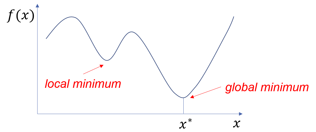
Finding the minimum of a function in 1D. See image description link below for full details. — **Figure 1**. Finding the minimum of a function in 1D.

The graph depicts two kinds of minima of a function with a single argument, a local minimum and a global minimum.

Please note: for accessibility purposes, detailed image descriptions are provided throughout the module adjacent to images that are too complex to be sufficiently described in alt-text.

For functions with n-dimensional input and a scalar output $f:\R^n\rightarrow\R$ find the value of $\myvec{x}$ that gives the minimum (or maximum) output from the function:

\[\myvec{x}^*=\underset{\myvec{x\in\R^n}} {\operatorname{argmin}}f(\myvec{x})\]

The diagram below illustrates the minimisation problem for $n=2$:

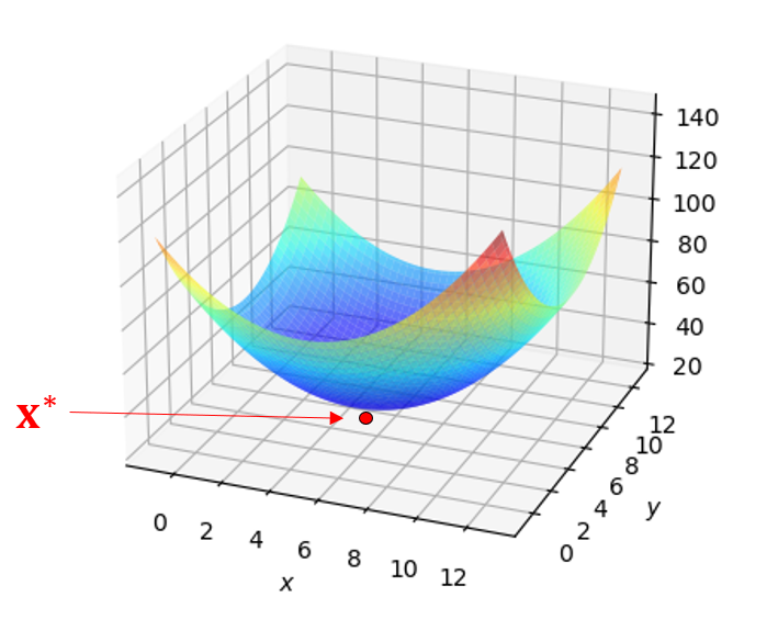
Finding the minimum of a function in 2D. See image description link below for full details. — **Figure 2.** Finding the minimum of a function in 2D.

A convex (bowl shaped) function of two arguments, showing a global minimum at the bottom of the bowl.

The simple form of the problem introduced at the start is equivalent to the multi-dimensional problem with $n=1$.

Gradient descent is a general method for finding the minimum of a function. The idea is to start with some random $\myvec{x}\in \R^n$ and make repeated small changes to $\myvec{x}$ in the direction of fastest decrease in $f(\myvec{x})$ at $\myvec{x}$. The following diagram illustrates this idea for $n=2$:

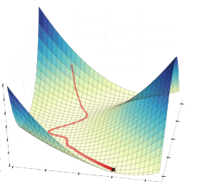
Image of 2-D surface and rolling down hill. — **Figure 3.** Illustrating gradient descent on a 2D function, showing the trajectory leading towards the minimum value.

The direction of fastest increase in $f$ is given by the gradient vector:

\[\nabla_\myvec{x} f(\myvec{x}) = \begin{bmatrix} \frac {\partial f}{\partial x_1} (\myvec{x})\\ \vdots \\ \frac {\partial f}{\partial x_n} (\myvec{x}) \end{bmatrix}\]

Note that the partial derivatives are evaluated for the given value of $\myvec{x}$.

Each of the partial derivatives in the gradient vector gives the ratio of the change in $f$ for an infinitesimal change in one of the components of $\myvec{x}$.

The magnitude of the gradient vector is the rate of increase in $f$.

Thus, in gradient descent we repeatedly make a small step from $\myvec{x}$ to a new point $\myvec{x'}$ defined as follows:

\[\myvec{x'}=\myvec{x}-\eta \nabla f(\myvec{x})\]

$\eta$ simply scales the step size and is generally a small number (e.g. $\eta=0.002$). Notice that the displacement is subtracted so that we move downhill.

For example, in 2-D suppose:

\[f(x,y)=3x^2+xy\]

The gradient vector with respect to $\myvec{x}$ is then given by:

\[\nabla_\myvec{x} f(x,y)=\begin{bmatrix} 6x+y \\ x \end {bmatrix}\]

Thus, the gradient vector at $(3,4)$ is $\begin{bmatrix} 22 \\ 3 \end {bmatrix}$. At $(2,3)$ the gradient vector is $\begin{bmatrix} 15 \\ 2 \end {bmatrix}$

For convenience, we will refer to partial derivative of the output with respect to the value at any intermediate node (including input nodes) as the gradient at that node.

Backpropagation

The functions we deal with in deep neural networks have many variables and a deep compositional structure. To compute gradients efficiently, we represent the evaluation of a given function as a computation graph (or computational graph). The computation graph is a Directed Acyclic Graph or DAG for short. For example, the evaluation of the function $e=(a+b)*(b+1)$ at $a=2, b=3$ can be represented as follows:

DAG for the example above. — **Figure 4.** The computation graph representing the evaluation of a simple 2D function.

A graph structure with five nodes, starting with the inputs a=2 and b=3 in two nodes on the left. Directed edges point from both of these 'input' nodes to a third node containing c=a+b, c=5. A single directed edge points from b=3 to a fourth node containing d=b+1, d=4. Nodes three and four are in the middle of the graph. On the right of the graph is a single output node with directed edges leading from the third and fourth nodes. This fifth node contains e=c*d, e=20.

This shows how the values of the input variables are mapped through intermediate steps to produce an output.

We will use this graph to compute gradients in an efficient way.

First, consider the special case of a function that is a composition of two elementary functions each taking a single argument, as in the following example:

Three nodes in a row labelled x, y and z, with a directed edge from x to y labelled with the partial derivative of y with respect to x, and from y to z labelled with the partial derivative of z with respect to y. — **Figure 5.** The chain of partial derivatives leading from x to z via y.

The derivatives between neighbouring variables are shown on the edges that link them. By virtue of the chain rule, the gradient at $x$ is simply the product of the two intermediate partial derivatives:

\[\frac{\partial z}{\partial x} = \frac{\partial z}{\partial y}\frac{\partial y}{\partial x}\]

An intuitive example of this is due to George Simmons [1]: "if a car travels twice as fast as a bicycle and the bicycle is four times as fast as a walking man, then the car travels 2 × 4 = 8 times as fast as the man."

For 'linear' compositions of more than two elementary functions, repeated application of the chain rule means that the gradient at any node is simply the product of partial derivatives on the edges between that node and the output node. The special case of the gradient for the input node is illustrated below:

\[\frac{\partial x_k}{\partial x_1} = \frac{\partial x_2}{\partial x_1} \cdots\frac{\partial x_{k-1}}{\partial x_{k-2}} \frac{\partial x_k}{\partial x_{k-1}}\]

Linear DAG. — **Figure 6.** Applying the chain rule to a composition of multiple functions.

A row of nodes connected left to right with directed edges between consecutive pairs of nodes. Partial derivatives between consecutive pairs of nodes are depicted as red arrows between the nodes. The partial derivative of the output node on the right with respect to the input node on the left is represented by a single red arrow leading from output to input.

The equation again for context:

$$\frac{\partial x_k}{\partial x_1} = \frac{\partial x_2}{\partial x_1} \cdots \frac{\partial x_{k-1}}{\partial x_{k-2}} \frac{\partial x_k}{\partial x_{k-1}} $$

Backpropagation computes such gradients by propagating backwards from the output, each time multiplying by the next edge derivative in the chain. The iteration is initialised by placing a gradient of 1 at the output node (i.e. $\frac{\partial x_k}{\partial x_k}=1$).

This iteration is expressed in the following algorithm:

**Figure 7.** Backpropagation algorithm for a chain of functions.

The output is node k. The partial derivative of node k with respect to itself is set to 1. The previous node is defined as node s. So long as s is greater than or equal to 1, set the partial derivative of node k with respect to node s as the product of the partial derivate of node s+1 with respect to node s, and the partial derivative of node k with respect to node s+1. decrement s and repeat. Note that on the first time through s+1=k.

For any tree-structured computation graph, we can propagate backwards in the same way, using the chain rule along the unique paths from the output (root) to the inputs (leaves). This is illustrated below:

Backpropagation in trees. — **Figure 8.** Backpropagation in a tree-structured computation graph.

A tree-structured DAG leading from 16 input nodes on the left to a single output node on the right. The backpropagation of the gradients from the output node to a single input node is illustrated by a curved path from right to left, passing via intermediate nodes in the tree. Such a path is shown for two of the input nodes.

Notice that the product that defines the gradient at any intermediate node of the tree is shared by all of the nodes (including leaf nodes) that can be reached via this node. Such products only need to be evaluated once.

In general, the computation graph may contain functions with two or more arguments that depend on the same variables from earlier in the computation graph, as in the graph below:

**Figure 9.** Multi-variable computation graph.

Here, there is more than one chain from $h$ to the output $z$. In such cases, we use a generalisation of the chain rule to:

\[ \frac{\partial z}{\partial h}=\frac{\partial z}{\partial x}\frac{\partial x}{\partial h}+ \frac{\partial z}{\partial y}\frac{\partial y}{\partial h} \]

Intuitively, we are adding the products from the two chains.

In general, the gradient at each node is the sum of all chain-products leading to the output. During backpropagation, we accumulate (sum) these contributions to the gradient.

Again, backpropagation computes all of these gradients efficiently by working backwards from the output, compounding the product of derivatives along every branch of the DAG and accumulating (adding) gradients at nodes that have multiple paths to the output. The sequence in which nodes are visiting during backpropagation is the reverse of the sequence they are visited during forward computation from inputs to the output. This guarantees that gradients are fully accumulated at intermediate nodes before we move on and backpropagate to earlier nodes.

Below, we see this process for the earlier example:

Illustrating backprogation. — **Figure 10.** Backpropagation for the computation graph in Figure 4.

The computation graph from Figure 4 is shown again. The partial derivatives between consecutive pairs of nodes are shown. For example, between node c and node e, the partial derivative is given by d, which is 4 (remember that e=c*d). The partial derivatives (gradients) of the output with respect to all nodes are shown in red at each node. Thus, the gradient at node a is the product of the gradient at node c and the partial derivative of node c with respect to node a (i.e. 4 = 1*4). At node b, the gradient is a sum of two gradients, that via node c and that via node d, giving 9 in total.

Functions of vectors

Often, the scalar variables in a computation graph will naturally group into array structures, for example a $256 \times 256$ array of light intensities that make up an image. It is convenient and efficient to express the computation graph in terms of such arrays and the elementary functions that operate on them. In machine learning, such arrays are referred to as tensors and may have several dimensions. A 1D tensor is a vector and 2D tensor is a matrix.

Consider the following example:

\[e=(\myvec{A}\myvec{x})^T(\myvec{x}+\myvec{y})\]

\[\myvec{A}=\begin{bmatrix} 1 & 1 \\ 2 & 2 \end{bmatrix}\]

We can represent this as a computation graph as follows:

**Figure 11.** Tensor computation graph.

A computation graph with five nodes. Two input nodes on the left have vector values: x=(1,2) and y=(3,5). The third node u=(3,6) (in the middle) is a function of x obtained bu pre-multiplying x by the square matrix A. The fourth node v=(4,7) (also in the middle) is defined as the sum of x and y. Finally, the fifth node e=54 (on the right) is an output scalar value obtained from the dot product of u and v.

Backpropagation on such computation graphs is analogous to the scalar case we've already considered. Suppose we have backpropagated to $\myvec{u}$ and now have the gradient $\begin{bmatrix} \frac{\partial e}{\partial u_1} & \frac{\partial e}{\partial u_2} \end{bmatrix}^T$. The implicit scalar computation graph underlying the elementary function at $\myvec{u}$ looks like this:

Underlying scalar graph with the components of x as two nodes on the left fully connected to the components of y as two nodes on the right. — **Figure 12.** The underlying scalar computation graph for a pair of vector nodes.

By the multi-variable chain rule, we propagate back to the components of $\myvec{x}$ as follows:

\[ \begin{bmatrix} \frac{\partial e}{\partial x_1} \\ \frac{\partial e}{\partial x_2} \end{bmatrix} = \begin{bmatrix} \frac{\partial u_1}{\partial x_1} \frac{\partial e}{\partial u_1} + \frac{\partial u_2}{\partial x_1} \frac{\partial e}{\partial u_2} \\ \frac{\partial u_1}{\partial x_2} \frac{\partial e}{\partial u_1} + \frac{\partial u_2}{\partial x_2} \frac{\partial e}{\partial u_2} \end{bmatrix} = \begin{bmatrix} \frac{\partial u_1}{\partial x_1} & \frac{\partial u_1}{\partial x_2} \\ \frac{\partial u_2}{\partial x_1} & \frac{\partial u_2}{\partial x_2} \end{bmatrix}^T \begin{bmatrix} \frac{\partial e}{\partial u_1} \\ \frac{\partial e}{\partial u_2} \end{bmatrix} \]

The $2 \times 2$ matrix in this equation is known as the Jacobian matrix. In general, for $\myvec{x}\in \mathbb{R}^n$ and $\myvec{u}\in \mathbb{R}^m$ we have:

\[\begin{bmatrix} \frac{\partial e}{\partial x_1} \\ \vdots \\ \frac{\partial e}{\partial x_n} \end{bmatrix} = \begin{bmatrix}\frac{\partial u_1}{\partial x_1} & \cdots & \frac{\partial u_1}{\partial x_n} \\ \vdots & \ddots & \vdots \\ \frac{\partial u_m}{\partial x_1} & \cdots & \frac{\partial u_m}{\partial x_n} \end{bmatrix}^T \begin{bmatrix} \frac{\partial e}{\partial u_1} \\ \vdots \\ \frac{\partial e}{\partial u_m} \end{bmatrix}\]

Here the Jacobian is a $m \times n$ matrix.

Remember that we must still accumulate gradients as we compute them to allow for different routes to the output. For example in the computation graph above, $\myvec{x}$ contributes to both $\myvec{u}$ and $\myvec{v}$, giving two routes to $e$.

Finally, vanilla gradient descent may not end up at a global minimum, particularly with function landscapes such as the following [2]:

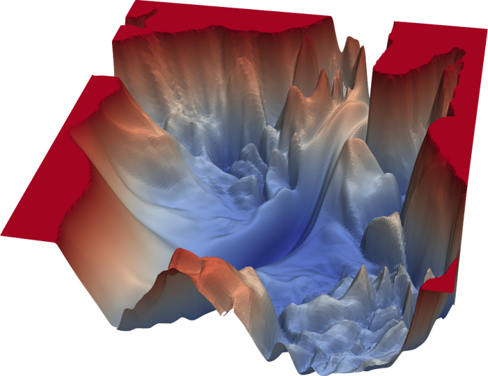
rough landscapes. — **Figure 13.** A 2D function with many local minima. This function is from an optimisation problem arising in deep learning and comes from Li et al. [2].

[1] George F. Simmons, Calculus with Analytic Geometry, McGraw-Hill, New York (1985), p93

[2] Hao Li, et al. Visualizing the Loss Landscape of Neural Nets, NeurIPS (2018), p6