Generative adversarial networks
We saw an example of a generative network in the section on RNNs. This was a generator of text. The input is a short segment of text and the network extends this text, character by character. The network implements an autoregressive process that defines a probability distribution over the vocabulary of possible next characters conditioned on the history of the output sequence up until the current timestep. In this section, we look at a different kind of generative network, where the aim is to generate examples from some domain, conditioned on a random vector sampled from a pre-defined probability distribution.
The aim is to build a generator of images from a given domain, such as outdoor scenes or faces, based only on a training set of example images from the domain. The typical setup is illustrated below:

Figure 1 The task of generating images from random vectors.
We sample a random vector \(\myvec{z}\) from some pre-defined distribution. This is input to a deep CNN that outputs a colour image \(\mymat{x}=g(\myvec{z})\) represented as a 3D tensor. The image is typical of images within a chosen domain, in this case outdoor scenes.
The random vector is drawn from a given distribution over \(\R^n\), where \(n\) is typically between 100 and 512. The random vectors are not specified as part of a training dataset and are therefore referred to as latent. Normally, the distribution decomposes so that the \(n\) components of each sample vector are drawn independently from the same 1-D probability distribution. Two common choices for this distribution are the normal (Gaussian) with mean 0 and standard deviation 1 (i.e. \(z \sim \mathcal{N}(0,1)\)), and the uniform distribution over the interval \([-1,1]\) (i.e. \(z \sim \mathcal{U}(-1,1)\)).
Here we will focus on the DCGAN [1]. The details of the DCGAN architecture vary depending on the resolution of image required as output. In experiments on generating images like those in the MNIST dataset, the architecture is as follows:

Figure 2 Architecture of the DCGAN generator.
The output of the first fully connected layer is reshaped to \(7 \times 7 \times 256\) as shown. The output images are \(28 \times 28\) intensity arrays (i.e. one channel deep). The progressive upsampling from \(7 \times 7\) to \(28 \times 28\) is achieved using fractionally-strided convolution. In regular (zero padded) convolution with stride \(n\), the output is \(n\) times smaller than the input. By contrast, convolution with a fractional stride of \(\frac{1}{n}\) makes the output n times larger by simply inserting \(n-1\) rows and columns of zeros between the rows and columns of the input to the convolution. The example below uses a \(3 \times 3\) kernel and a fractional stride of \(\frac{1}{2}\).
Figure 3 Convolution with a fractional stride of 1/2.
The Leaky ReLU function is a modification of ReLU to replace the flat zero output for negative inputs by a positive gradient. This still attenuates negative inputs, but avoids zero gradients, which contribute nothing to gradient descent. The slope of the line would typically be around 0.1 (i.e. \(a=0.1\)). It is also possible to learn an optimal value for \(a\) as part of the training.

Figure 4 Graph of the leaky rectified linear unit function.
Training
The training data is a set of images from the target domain. If we knew the latent vector corresponding to each of these images, this would be a conventional supervised setting with paired data of the form \(\{(\myvec{z}_i,\mymat{x}_i)\}\). Without the corresponding latent vectors, the problem is partially supervised to the extent that we are given examples of images \(\{\mymat{x}_i\}\) from the target domain but no more. In this situation, the question is what do we do for a loss function?
In the approach adopted for Generative Adversarial Networks (GANs), the solution is to use a regular CNN classifier (the discriminator) as a loss function to train the generator. The classifier outputs a probability \(d(\mymat{x})\) that an input image is real (i.e. from the target domain). The probability that the image is fake (i.e. from the generator) is then simply given by \(1-d(\mymat{x})\). The parameter values of the discriminator are updated in a regular supervised setting to increase the log likelihood on a minibatch of \(m\) images \(\{\mymat{x}^{(1)},\cdots.\mymat{x}^{(m)}\}\) from the chosen domain and fake images from the generator \(\{ g(\mymat{z}^{(1)}),\cdots.g(\mymat{z}^{(m)})\}\), obtained from a sample of \(m\) latent vectors \(\{\mymat{z}^{(1)},\cdots.\mymat{z}^{(m)}\}\). The log likelihood objective is given by:
where we are seeking to update the parameters values of the discriminator \(\boldsymbol\theta_d\).
Note that in a GAN, the discriminator is only updated for one or a small number of iterations at a time.
We now switch to updating the generator. To do this, we could generate another sample of \(m\) latent vectors and pass these through the generator to give a new set of fake images. In DCGAN, this isn't done, and instead the previous set of fake images is re-used (you will see this in the PyTorch tutorial later in this lesson). The discriminator can now be used as the basis of a loss function for training the generator. We impose the label 'real' for each of the fake images. Again this provides a regular supervised setting, with only fake images as input, all labelled 'real'. The log likelihood to be maximised now becomes:
The second term in (6.1) associated with the 'fake' class disappears since we only have images labelled 'real'.
The rationale here is that we are updating the generator to increase the log probability of the 'real' class on fake images. In other words, the generator is improved such that its output images are more likely to be labelled as 'real'.
The gradients of the log likelihood are backpropagated through the discriminator and then through the generator. Only the parameter values of the generator are updated; those of the discriminator remain fixed.

Figure 5 Training the generative network.
The architecture of the discriminator in DCGAN is as follows:

Figure 6 Architecture of the DCGAN discriminator.
This is a simple classifier with two convolutional layers and a single scalar \(d(\mymat{x})\) as output - the probability that the input image \(\mymat{x}\) is real.
Because the generator is now doing a better job of producing images that look like those from the chosen domain, we return to updating the discriminator as before. Having updated the discriminator, we return again to updating the generator and so on until the discriminator is unable to tell the difference between fake and real images. Thus, the generator and discriminator improve together, minibatch by minibatch.
In summary, the method is as follows:
Initialise the generator and discriminator networks randomly from a normal distribution

  Repeat num_epoch times

    Repeat on each batch of real images

      Sample from latent distribution and use generator to produce a batch of fake images

      Update discriminator to increase the log likelihood
          on the output from real and fake images (equivalent to using cross-entropy loss)

      Pass fake images through the current discriminator to generate output probabilities

      Backpropagate gradient through discriminator and generator, and update generator
          to increase the log likelihood of 'real' for the fake images.
Adversarial setting
In this iterative method, the generator and discriminator can be viewed as competing with one another. This can be couched as a zero-sum game with payoff \(v(\boldsymbol\theta_g,\boldsymbol\theta_d)\) to the discriminator given by:
where \(\theta_g\) and \(\theta_d\) are the parameter values of the generator and discriminator networks.
The first term is the expected value of the log probability of \(\mymat{x}\) being real, given \(\mymat{x}\) distributed as \(p_{data}\), the distribution of real images. The second term is the expected value of the log probability of \(\mymat{x}\) being fake, given \(\mymat{x}\) distributed as \(p_{model}\), the distribution of fake images.
In updating the discriminator, we seek to maximise the payoff. Since this is a zero-sum game, the payoff to the generator is simply \(-v(\boldsymbol\theta_g,\boldsymbol\theta_d)\). Thus we update the generator to decrease \(v(\boldsymbol\theta_g,\boldsymbol\theta_d)\). The turn-taking of the game is repeated until convergence, when the optimal generator is given by:
In this minimax formulation, the optimal generator minimises the maximum payoffs achieved by the discriminator.
Under certain general assumptions on the form of \(g\) and \(d\), it can be shown that the game will eventually converge on this optimal generator. However, when the discriminator and generator are implemented as multi-layer neural networks, as in DCGAN, the general assumptions don't hold in general and convergence can't be guaranteed.
In implementing this adversarial approach, the expected values in the payoff are estimated on minibatches of real and fake images. The estimate is simply the log likelihood defined in \((6.1)\) above and used in DCGAN to update the discriminator.
In practice, updating the generator to decrease the payoff \(v(\boldsymbol\theta_g,\boldsymbol\theta_d)\) doesn't work as well as updating the generator to increase the chance that the discriminator makes a mistake on fake images, defined as the expected value \(\mathbb{E}_{\mymat{x} \sim p_{model}} \log(d(\mymat{x}))\).
This is the basis on which the generator for DCGAN is updated, giving rise to the estimate of this expected value on a minibatch in \((6.2)\) above.
Results
The following animation shows the images generated from a fixed sample of latent vectors over 50 training epochs.
Figure 7 Animation of the improvement in the generator over time. 16 latent vectors are sampled before training begins; the images generated from these vectors are shown after each epoch. The images begin as random noise and become increasingly recognisable as written digits. This animation is from the tensor flow tutorial on DCGAN .
The following figure shows fake images from a generator trained on 3 million images of bedrooms:
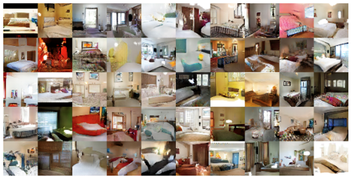
Figure 8 Fake images of bedrooms.
From Radford et al. [1]
It is interesting to observe the way in which generated images change as we make a tour of the latent space. In the following illustration, nine latent vectors have been sampled at random, from which intermediate points are generated by interpolation. The result is a trajectory through the latent space consisting of a sequence of 100 latent vectors, from which a corresponding sequence of slowly changing images is generated. The 100 images are shown in order scanning left to right from top to bottom. Notice that the contents of the bedrooms change smoothly as we transition through the 100 images.
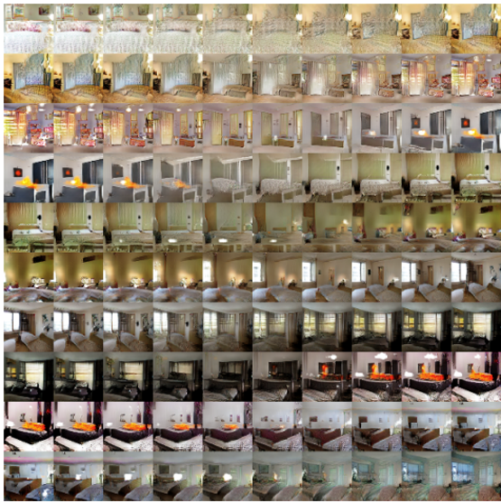
Figure 9 Touring the latent space.
From Radford et al. [1]
Tutorial
There is an implementation of DCGAN available as a
PyTorch tutorial. Please go through this tutorial. Having understood the
explanation above, you should be able to follow the code,
looking in particular at the definition of the two models
Generator and Discriminator, and the
section on Training. You can download the notebook, or run in
Colab directly from the tutorial.
The dataset file is called img_align_celeba.zip and sits within the img directory in the shared area accessed from the 'Align&Cropped Images' download shown on the front page. The dataset required is 1.34Gb as a ZIP file so takes a while to unzip.
BigGAN-deep
We now look at a much larger generator network developed by Brook et al. [2]. The architecture of BigGAN-deep is shown below:

Figure 10 Architecture of BigGAN-deep.
Based on a diagram from Brock et al. [2]
The input is the concatenation of a random vector \(\myvec{z} \in \R^{128}\) and a \(128D\) embedding of the desired class. The embedding is a lookup table from the class index to a \(128D\) embedding vector, but can also be implemented as a linear function of the one-hot encoding for the class index. Either way, the embedding can be learnt as part of the training. The \(256D\) vector that results from concatenation is passed through a linear mapping and reshaped to \(4\times 4\times 16\) channels. This is followed by four residual blocks, each containing multiple convolutional layers, with upsampling and batch normalisation. Notice that the input is supplied into each of the residual blocks. After training the generator on ImageNet using an adversarial loss (as for DCGAN), \(256\times 256\) resolution images like those shown below are produced by sampling from the latent space and selecting a desired object category.
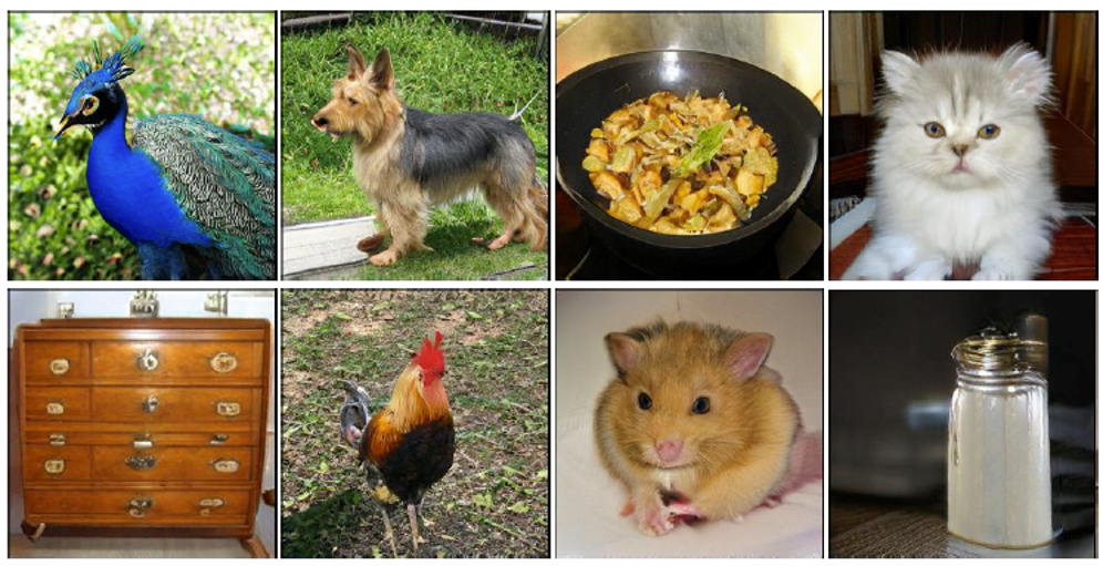
Figure 11 Examples from BigGAN-deep trainined on ImageNet.
From Brock et al. [2]