Convolution
Image smoothing using cross-correlation
There is often a need to smooth the intensity values over the pixels that make up an image. Smoothing can remove small scale detail such as random noise. To illustrate this, consider a 2D array (matrix) of mean intensity values obtained by taking the mean of the red, green and blue colour channels at each pixel.
For the colour image on the left, the mean intensity image is depicted on the right, rendered using a grey colour map. Remember that displaying an image requires three values for each pixel: the RGB values. The colour map defines these values for shades of grey in the interval [0,1].
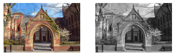
Figure 1. From a colour image (left), generate a mean intensity image and display using a grey colormap (right).
A simple way to smooth the image is to replace the value at each pixel by the mean of the neighbouring values (including the current pixel). This can be computed using a \(3\times 3\) array (referred to as a kernel or mask) containing the value \(\frac{1}{9}\) in each location.

Figure 2. A 3x3 kernel for smoothing an image.
The centre of the kernel is placed at each location of the image. Each value in the kernel is then multiplied by the value beneath and the resulting products are summed, with this value being inserted into a new image at the corresponding position. We refer to this process as cross-correlation.
The process is nicely illustrated by these animations from: https://github.com/vdumoulin/conv_arithmetic
Figure 3. Illustration of correlation with no padding.
Because the kernel can't be centred on the boundary rows and columns of the image, there are fewer rows and columns in the output than the input. To make the output image the same size as the input, it is common practice to expand the original image with additional rows and columns on the left and right and on the top and bottom. This means that the kernel can be centred at all pixels locations of the original image. The additional rows and columns are normally filled with zeros.
Figure 4. Illustration of correlation with zero padding.
Two variations of the procedure are to move the kernel one or more steps at a time across the columns and down the rows. We call the step size the stride. For example, in the following correlation with zero padding, the stride is two.
Figure 5. Illustration of correlation with stride of 2.
Another variation is to interspace the values in the kernel as they are applied to the image values. We refer to the degree of interspacing as the dilation. For example, in the following illustration the dilation is two.
Figure 6. Illustration of correlation with dilation of 2.
The result of cross-correlation of an image \(f(x,y)\) with a kernel \(h(u,v), -1 \le u,v \le 1\) can be expressed as:
In practice, to smooth an image, the kernel will normally have the shape of a 2-D Gaussian function, which gives more emphasis to the centre values and progressively less emphasis away from the centre. The definition of a 2-D Gaussian function centred about the origin is as follows:
This is defined over the whole of the u-v plane (out to infinity) such that the area underneath the surface sums to one. To build an nxn kernel from this function, we sample at integer values over an nxn grid. To smooth the image without brightening or darkening the result, it is important the weights add up to one. To ensure this is the case, we normalise the kernel by dividing every weight by the sum of the weights. Such a kernel is shown below, where each of the values should be multiplied by 0.001 as illustrated:

Figure 7. Gaussian weights in a 5x5 kernel.
The amount of smoothing is determined by the spread of the Gaussian. This spread is controlled by the value of \(\sigma\) (sigma). This is also the standard deviation of the Gaussian. The following diagram shows the result of correlation with a Gaussian kernel for three different standard deviations.
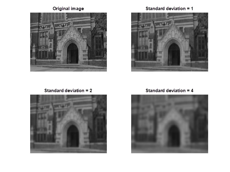
Figure 8. Correlation with Gaussian kernels for standard deviations 1, 2 and 4.
The three corresponding kernels are illustrated in the diagram below:
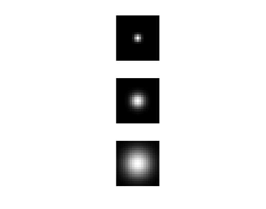
Figure 9. Three Gaussian kernels used for the smoothing depicted in Figure 8.
Convolution
If we rotate the kernel by a half turn (180 degrees) before applying cross-correlation, the resulting operation is known as convolution. The convolution of an image \(f\) with a kernel \(h\) is written as \(h*f\) for short.
Note that a Gaussian kernel of the form above is invariant under any rotation. Therefore cross-correlation and convolution with a Gaussian kernel amount to the same thing.
From now on, we will refer to the process as convolution.
Retinotopic maps in natural vision systems
The process of convolution computes a new value at each location from local values according to the scalar values in the kernel. The local nature of this computation is mirrored in the human visual system. This is illustrated in experiments reported in 2003 by Dougherty et al. [1].
The visual cortex at the back of the brain contains regions of neural cells (neurons) that seem to be laid out in correspondence with the visual field (image received by the eye). Functional magnetic resonance imaging (fMRI) is used to produce images of the brain where pixel intensities correspond to blood flow, which in turn is a measure of the activity levels of neurons. These regions are referred to as retinotopic maps. In an experiment with human subjects, a circular chequered pattern (shown top-left in the figure below) expands in an outward direction. As the chequered pattern moves over the visual field, different parts of the visual cortex become stimulated. Remarkably, the areas of stimulation seem to be organised as maps in correspondence with the retinal images. We call these retinotopic maps. In the diagram below, the surface of the cortex is colour coded with the size of annulus that stimulates that location.
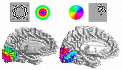
Figure 10. Functional magnetic resonance images showing localised response to expanding and rotating stimuli.
From Dougherty et al., 2003 [1].
The colour coding is shown to the right of the displayed pattern. Similarly, a rotating pattern (top-right), and associated colour coding, causes a gradual variation orthogonal to the first in the visual cortex (bottom-right image). A given location in this region of the cortex therefore corresponds with a specific radial distance and angle of a stimulus falling onto the retina. In other words, it provides polar coordinates for the stimulus.

Figure 11. Polar coordinates represent the position of a point as an angle and a distance from the origin.
Overall, this region of the visual cortex is in one-to-one correspondence with the retinal; it is a retinotopic map.
In the diagram below, nine retinotopic maps can be seen in the visual cortex. Area V1 is known as the primary visual cortex.
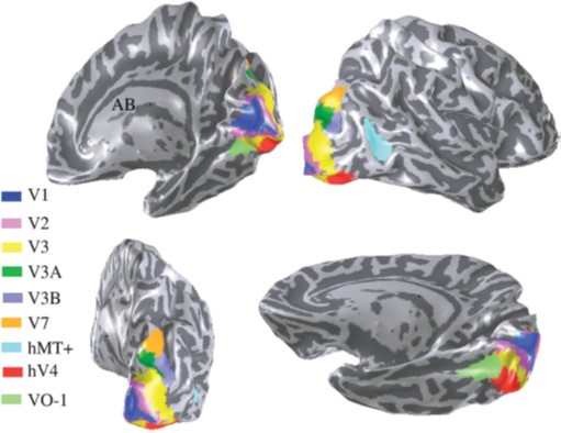
Figure 12. The locations of nine retinopic maps.
From Wandell et al. [2].
Four views of the visual cortex showing nine colour-coded regions where there are retinotopic maps.
An original set of experiments from the pioneering work of Hubel and Wiesel in 1960 [3] used electrical probes to measure the activity in different clusters of neurons within the visual cortex of animals in response to different kinds of stimulus.
These experiments indicated that the brain contains neurons that fire more rapidly when specific visual patterns appear at fixed locations in the visual field. Some cells respond to intensity edges in specific orientations, and others to bar shapes in specific orientations. Some cells only respond to edges or bars that are moving ‘sideways’ across the visual field.
Here is an original video of this work.
From work like this, the visual cortex seems to be producing maps for different visual features present in the visual field. We refer to these as feature maps. We now know that the brain adapts the patterns detected to the patterns that are observed in the visual field – we might say that the patterns are learned. This property of the neural apparatus is referred to as plasticity.
It turns out that such maps can be easily produced using convolution with appropriately chosen kernels. Moreover, we can learn the values in these kernels from natural images.
Feature detection using convolution
The following images have been obtained by convolving the arch image with the four \(3 \times 3\) kernels shown above each image. Locations in the image for which the value computed by convolution is above 0.5 are shown in white. The four convolutions produce the highest values for intensity edges in four orientations. The vertical structure in the arch is visible with the top two kernels and the horizontal structure elsewhere is visible with the bottom two kernels. In fact, one of the vertical convolutions could be obtained by negating the sign of the other vertical convolution and likewise for the pair of vertical convolutions. However, we have retained all four convolutions to emphasise the difference in the patterns of image intensity. The kernels used here are normally associated with the name Sobel from the early days of computer vision.

Figure 13. The four images show locations where there is a large positive response to convolution with the 3x3 kernel shown above each image.
The following image shows the strongest response from the four convolutions at each pixel location using a unique colour for each kernel (shown in the corners of the images above).

Figure 14. The dominant response of the four convolutions at each location, using a unique colour for each kernel.
References
[3] D N Hubel and T H Wiesel (1960), Journal of Physiology, 160.