Convolutional neural networks
A convolutional neural network applied to images is organised as a series of layers. Each layer uses convolution to produce a set of feature maps using a different kernel for each feature map. The feature maps from one layer are passed as input to the next layer. The first layer receives the image as input. By analogy with fully-connected layers, a single bias value is added to every value in each feature map. This bias value will normally be different for each feature map.
For RGB images there are three colour channels on input. To deal with this, a separate convolution is applied to each channel, normally with different \(m \times m\) kernels. The results are then added pixelwise to produce a single 2D output. Finally, we add a single scalar bias value and the result is an output feature map.

Figure 1. A separate convolution applied to each colour channel contributes to the values in the output feature map.
An alternative way of looking at this is that we are performing a single 3D convolution with a \(3 \times m \times m\) kernel on the full 3D (RGB) input tensor. This 3D kernel is simply a concatenation of the three 2D kernels along the first dimension. In this operation, the kernel is applied at every spatial location, spanning all three channels. We don't scan the kernel in the first dimension because it has only one position in this dimension that keeps it within the 3D input tensor. In general, the output from a 3D convolution would be 3D, but in this case it is only one layer deep and can therefore be considered to be a 2D array - the result we require.

Figure 2. The convolutional layer applied to an RGB image can be viewed as a single convolution with 3D kernel applied to the 3D image tensor.
Conceptually, we can think of the convolution as looking for image features that involve all three colour channels. Thus, for example we might find a detector that is sensitive to vertical edges, separating red and green regions of the image.
The whole process can be repeated as many times as we wish using different 3D kernels and generating different feature maps on output. Note that we normally use a different bias value for each feature map.
In summary, we take a 3D tensor as input with three colour channels and output an 3D tensor as output, with \(K\) feature map channels. For convenience we refer to the number of channels as the depth of the tensor, as opposed to its spatial dimensions of width and height.
For subsequent layers of the CNN, we simply apply the same process, except that the input to a layer may contain any number of channels (\(K \times h \times w\)), which are either the feature maps from the previous layer or the three colour channels of the input image. In general, the kernel will be \(K \times m \times m\) in size. As for a regular multi-layer network, the layers are separated by a non-linearity to accentuate the strong responses. You can think of the layers of the CNN as forming spatial features from the prominent features detected in the previous layer. As we move up the layers, the features become more and more complex, starting out with simple features of the image and ending up with features that might correspond to parts of an object, or indeed a whole object.
In convolution, each output value comes from the weighted sum of values in a window onto the input image. The weights remain the same for every output position. This is in contrast to a fully-connected linear layer where each output value comes from a unique weighted sum of all (flattened) input values.
Pooling
A so-called pooling layer is used in CNNs to reduce the spatial size of the feature maps and give some invariance to small spatial transformations of the input image, which might arise from small translations or deformations. The idea is to tile the feature map with a fixed sized window and then to aggregate the values in the window at each position into a single scalar value. The idea is that the aggregate value provides a summary the values within the window. In max-pooling this is the maximum of the values. For translations of the image smaller than the size of the window, this maximum value will often remain the same.
Normally the tiles sit side-by-side in rows and columns, but they may also overlap. As for convolution, the arrangement is specified by an integer stride. Thus, the following arrangement for max-pooling is specified by a \(2 \times 2\) window and a stride of 2.

Figure 3. Illustrating max-pooling with a 2x2 window and stride of 2.
Note that a translation of the image by one pixel to the right or one pixel up keeps the maximum value from the upper-left tile as '7'. On the other hand, a translation of the image by one pixel to the left will replace the maximum value in the upper-left tile by '4'. In this case, the invariance of the max-pooling to one-pixel translations is only partial.
The pooling layer normally reduces the size of the feature map. In the above case, the width and height are reduced by a factor of two.
A CNN for image classification
We are now ready to use a CNN for image classification. The following diagram illustrates the architecture of a CNN with two convolutional layers by focusing on the size of the intermediate tensors. Each of the convolutional layers is followed by max-pooling. The output from the final max-pooling is flattened, meaning that all of the values in the 3D tensor are concatenated into a single vector. It doesn't matter the order in which this occurs, providing it is done consistently. A final fully-connected layer converts this vector into a vector of class confidence values, which is in turn mapped into class probabilities using softmax (see Linear classifier).

Figure 4. The data flow of a CNN with two convolutional layers and a single fully connected layer leading to a probability distribution over ten classes.
The data flow diagram shows three 64x64 colour channel images at the left, passing through a convolution layer into 4 64x64 feature maps, a max-pooling layer into 4 32x32 feature maps, another convolutional layer into 8 32x32 feature maps, another max-pooling into 8 16x16 feature maps, flattening of the feature maps into a vector of size 2048, and finally a fully-connected layer into a vector of size 10, with softmax at the end.
A different representation of the same CNN architecture is shown below. This time we focus on the functions applied at each layer and give the tensor sizes on the connections.

Figure 5. Alternative data flow diagram for the CNN depicted in Figure 4.
The data flow diagram gives more information on the individual steps. The two convolutions use 3x3 kernels, with a stride of 1 and zero padding.
This CNN has many parameter values that must be estimated during optimisation on a training dataset. It is instructive to count the number of these parameters. We must include the convolutional kernels, bias values and weights in the fully connected linear layer. The number of such parameters are shown below:

Figure 6. The number of parameters associated with each step of the architecture shown in Figure 5.
The first convolutional layer has 3 (in channels) x 4 (out channels) x 9 (weights per kernel) + 4 (bias values) = 112. The two max-pooling layers and flatten layer have no parameters. The second convolutional layer has 4x8x9+8=296 parameters. The fully connected layer has 2048 (in) x 10 (out) + 10 bias values=20490. This gives 20898 parameters in total.
Notice that the number of parameters associated with the two convolutional layers is much lower than for the fully-connected 'classifier' layer. Intuitively this seems reasonable. The convolutional layers are responding to common features of the objects depicted in the domain and there should be sharing of features between object classes. On the other hand, the final classifier layer has to deal with assembling the features for each object class independently. It also has to cope with the natural variation in the appearance of an object within the image (i.e. position, orientation, scale, deformation, within class variation).
Training
We train the network on a given dataset in the same way as for our multilayer networks, using gradient descent on minibatches with gradients computed via backpropagation.
In PyTorch, this adds a new dimension in the first position of the input, giving a 4D tensor of size \((N,C,H,W)\) where \(N\) is the number of 2D inputs, \(C\) is the number of channels, and \(H,W\) are the number of rows and columns in each 2D input. The individual convolutional layers then progressively process the whole minibatch until the loss function can be computed at the end.
In terms of our running example, the input and output tensors at each level would be as follows:

Figure 7. Network architecture showing the tensor size at each stage.
Typically, we don't show the extra dimension when visualising a network since it is secondary to the conceptual operation on a single input at a time.
During training we collect statistics on how the loss function and accuracy computed on the training and test data changes over each epoch (i.e. each iteration of gradient descent on the complete training dataset). In the following graph, we see how the loss and the accuracy statistics change in one such experiment on the CIFAR-10 dataset. Notice that the loss and accuracy continue improving with each epoch on the training data, yet performance levels-off prematurely on the test data. This is a sign that the network is over-fitting to the training data.

Figure 8. Training and test loss and accuracy over 50 epochs. Notice that the test accuracy levels out well below the training accuracy, and the test loss starts to increase as the training loss continues to decrease. This is a sure sign of over-fitting to the training data.
In evaluation mode, we are simply interested in computing the outputs from individual inputs. For efficiency, it makes sense to group this computation into minibatches as would be done during training, but we don't need to build a computational graph since there is no need for gradients.
Data augmentation
One way to avoid over-fitting is to the reduce the capacity of the model to do this by lowering the model complexity, thereby reducing the number of parameters.
Another way is to increase the size of the training set. A major step in this direction can be achieved by data augmentation in which new input images are produced by:
- applying random transformations to the images in the training set.
- simulating changes in camera position and orientation by translating.
- rotating and scaling the image.
- scene lighting by scaling intensity values.
- intraclass variations in shape and appearance by applying small image deformations.
The new images come pre-labelled with the label from the image from which each new image is obtained. A series of such transformations are shown below.

Figure 9. Four transformations of an image from the dataset. Each of the resulting images can be used to augment the dataset during training.
In the following generated images random transformations have been combined and applied to a single image. The component transformations are to rotate, translate, scale, flip and alter the saturation/hue/brightness of the original image.
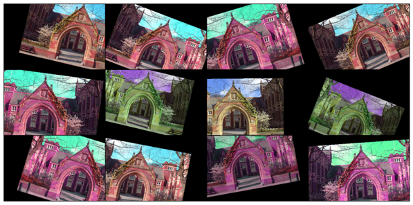
Figure 10. Random compositions of elementary transformations applied to an image.
Dropout
A third way to avoid over-fitting is to apply a process known as dropout. The idea is to perturb training examples, not by transforming the input image, but by zeroing input values to a layer with some given probability \(p\). We are effectively removing features at a chosen layer in the CNN. Dropout is a form of regularisation that can reduce generalisation error and thereby improve performance on unseen data.
Batch normalisation
Training can often be improved by reducing the variability of the data using batch normalisation. Here we normalise the values in the input image, or in feature maps, by standardising over each batch of data. The normalisation of a value within a feature map is based on the mean and standard deviation of all values in the corresponding feature map across the whole batch. Thus, it is sometimes called spatial batch normalisation. Thus given an input of size \((N,C,H,W)\) we normalise every value \(x\) from channel \(c\) as follows:
where the mean value for channel \(c\) is given by \(\mu_c = \frac{1}{NHW} \sum_{n=1}^{n=N}\sum_{h=1}^{h=H}\sum_{w=1}^{w=W} x_{n,h,w}\) where \(x_{n,h,w}\) is the value in row and column \(h,w\) of input \(n\) in the minibatch.
The standard deviation is computed in an analagous fashion.
Note that batch normalisation is faciliated by the way in which layers work on a whole minibatch at once.
In a final step, a channel dependent affine function is applied to \(x'\) so that the final output of batch normalisation is given by:
The values of these (\(2C\)) parameters are typically included in the optimisation. Notice that if we chose \(\alpha_c = \sigma_c\) and \(\beta_c = \mu_c\) the normalisation step is undone and \(y=x\) ! The idea is that the optimisation will find whatever are the best values, even if this means undoing the normalisation. In PyTorch, the parameters of the affine transformation are learnable by default.
Finally, in evaluation mode when we are applying the CNN to a single input, there may be no minibatch of data to normalise over. In this case, we simply use a mean and standard deviation that has been carried over from the training data.
Receptive fields
In a CNN, the value at each posiiton in a feature map derives from a region of values in the input image known as the receptive field for that feature map position. Typically the size of the receptive fields grows as we move through the layers of the CNN.
Consider the following CNN:

Figure 11. A simple CNN with the receptive field size at each stage.
A CNN architecture consisting of convolution with a 3x3 kernel, followed by a convolution with a 4x4 kernel, followed by 2x2 max-pooling with a stride of 2. The corresponding receptive fields are 3x3 following the first convolution, 6x6 following the second convolution and 7x7 following the max-pooling.
The \(3 \times 3\) convolution in the first layer produces a receptive field of size \(3 \times 3\). The receptive field size following the second layer \(4 \times 4\) convolution grows to \(6 \times 6\), meaning that each value in the resulting feature map is determined by the values in a \(6 \times 6\) window in the input image. This can be seen from the following illustration showing the \(3 \times 3\) receptive fields of four values along the diagonal of a \(4 \times 4\) window that combine to give an output value from the second layer.

Figure 12. Receptive field of 6x6 arising from convolution with a 3x3 kernel followed by convolution with a 4x4 kernel.
These three receptive fields span a \(6 \times 6\) window in the input image.
The \(2 \times 2\) maxpooling layer results in output values with a receptive field size of \(7 \times 7\) as a direct result of there being two adjacent \(6 \times 6\) receptive fields from the layer below in both rows and columns.

Figure 13. Receptive field of 7x7 arising from 2x2 max-pooling of values each having a receptive field of size 6x6.
Network visualisation
By examining the feature maps and kernels in a deep classifier, we can find out something about the function of these maps and thereby shed light on how the deep network is working.
In this section, we will be examining the feature maps and kernels obtained from one of the earliest CNNs known as Alexnet [1], trained on 1000 object classes from ImageNet.
Grad-Cam
The Grad-Cam method is a way to find out which parts of an input image contribute most to selection of a given class label. Consider the image below:
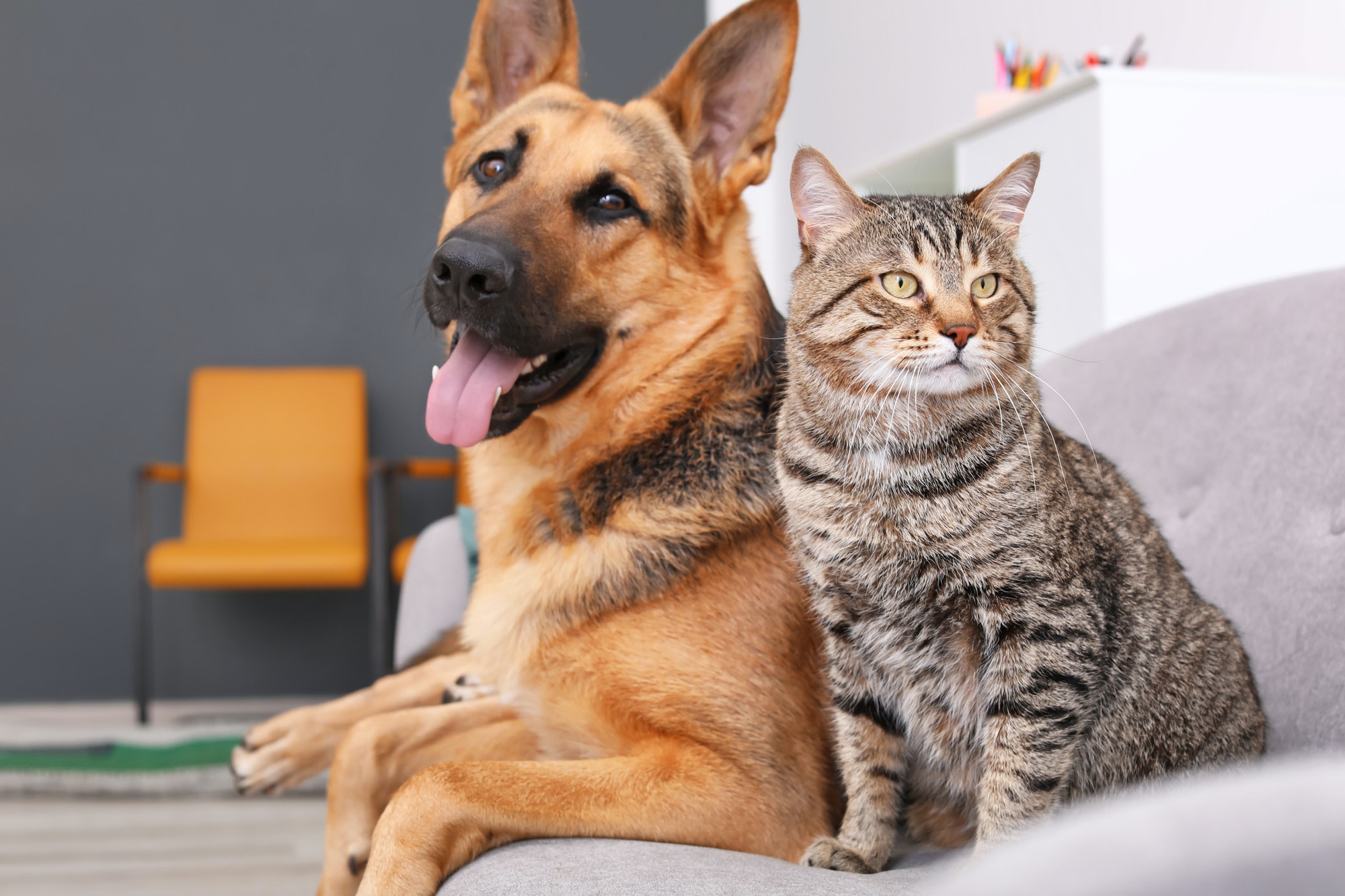
Figure 14. Which parts of this image are most important for a classifier in detecting the German Shepherd dog, and the Tabby cat?
For the classifier Alexnet trained on ImageNet, the Grad-Cam method produces the following result given the class 'Tabby cat':
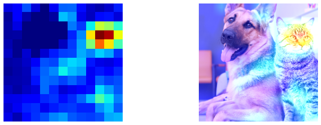
Figure 15. For the output class 'Tabby cat' the Grad-Cam method highlights the head of the cat.
Given the class 'German Shepherd', Grad-Cam generates the following:
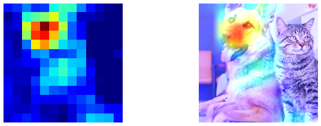
Figure 16. For the output class 'German Shepherd' the Grad-Cam method highlights the head of the dog.
This is of course highly intuitive and helps to confirm that the network is doing something sensible.
Grad-Cam works as follows. We run the network in evaluation mode on a test image and select the class label for a prominent object. We then backpropagate the gradient from the scalar confidence value for the target class \(y^c\) to the feature maps (activation maps) output from the final convolutional layer. These gradients form a 3D tensor \(\frac{\partial y^c}{\partial \mymat{A}}\) of size \(C \times H \times W\) and give an indication of the extent to which each spatial location contributes to variation of the output label confidence \(c\). We assume that each \(W \times H\) 2D feature map \(\mymat{A}^k\) making up \(\mymat{A}\) is sensitive to the patterns of activation associated with one or more object classes (e.g. Tabby cat). Furthermore, because of the translational invariance of the convolutional structure giving rise to the feature map, the location of an object instance within the image will be mirrored in regions of high activation within the feature map and within the gradient map. For the chosen class confidence \(y^c\), we sum the gradients for each feature map to give an average gradient for each feature map:
Intuitively, higher values of \(\alpha_k^c\) are obtained for features maps that are most influential in deriving the confidence for the target class \(c\). Finally, we now compute a weighted sum of the feature maps and apply the ReLU activation function to suppress negative values:
Inspecting the kernels
We can also visualise the convolution kernels that are learnt during training. For Alexnet trained on ImageNet, the kernels in the first convolutional layer are \(11 \times 11\). This is large enough to provide a discernible pattern when viewed as an image. If we normalise the values of the learnt kernels in the trained Alexnet into the range \([0,1]\) we obtain the following 64 kernels - one for each of the output feature maps. For visualisation purposes, the 3D kernels are rendered in colour, treating the depth dimension as RGB colour channels. Note that the kernels resemble the features that they respond most strongly to in the image. This is simply because the dot product computed by the vectorised kernel and image values at each location in convolution produces a measure of similarity between vectors when they are suitably normalised. As expected, the spatial patterns are reminiscent of the receptive fields discovered by Hubel and Wiesel. There are features in different orientations and with different colour contrasts.
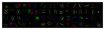
Figure 17. The 64 by 3 channel 11x11 kernels from the first convolutional layer of the pre-trained Alexnet, visualised by combining each set of three corresponding channels to form an RGB image.
Note: the pre-trained version of Alexnet available via torchvision has 64 feature maps from the first convolutional layer. The original Alexnet had 96.
Reference