Transformers
The transformer architecture was first proposed by Vaswani et al. in 2017 [1]. We will be looking at this model architecture in the section on the 'Full transformer' below. However, we start with the transformer used for the series of GPT systems built by Open-AI and first reported in a preprint by Radford et al. in 2018 [2].
The model from Radford et al. [2] is a seq2seq mapping function used for language modelling. The system can be used for text generation in a similar setup to an RNN, except that the network is not recurrent and input and output sequences are fixed length.
The overall architecture looks like this:

Figure 1. Transformer architecture.
Input encoding
The input is a context sequence of \(seqlen\) tokens (in GPT3 \(seqlen=2048\)). In handling text, the tokens could represent words, characters or fragments of words. In Generative pre-training (GPT), a commonly occurring set of word fragments is chosen in order to provide a compact encoding of raw text input. For example, 'The cat sat on the mat' might be encoded as:
Note that the spaces between words have been included in the encoding, represented here by the '_' symbol. The approach taken here is an example of Byte Pair Encoding (BPE). Starting with individual characters as our set of tokens, we recursively merge the most commonly occurring pairs of consecutive tokens and replace with new tokens representing those pairs. In GPT, there are 256 basic characters, merged recursively 50,000 times to represent longer and longer character sequences, each with a new unique token. This gives a total of 50,257 possible tokens: 256 basic tokens, 50,000 tokens arising from pairwise merging, and a special end-of-text token.
We now use an embedding to turn the 1-D vector of tokens representing a text string into a 2D tensor of size \(seqlen \times d\), where \(d\) is the length of each embedding vector (in GPT1 \(d=512\)). The embedding could come from word2vec on a corpus of text and working with fragments of words instead of whole words or individual characters. The input layer and embedding layer are shown at the bottom of Figure 4.1.
Multi-head attention
The most key part of the transformer architecture is the multi-head attention.
The terminology used to describe this step comes from the data retrieval literature. A database consists of a set of (key, value) pairs. Given a query, we retrieve a desired value by finding the closest key to the query. In our 'attention' context, queries, keys and values are all vectors. Given a query value, we measure the similarity to every key vector. We then sum all value vectors, weighted by the corresponding similarities. The idea is that the attention mechanism is focusing on those values associated with the most similar keys to the query.
The similarity between query vector \(\myvec{q}\) and key vector \(\myvec{k}\) is measured using the dot product: \(\myvec{q} \cdot \myvec{k}\). For efficiency, we pack the query, key and value vectors into the matrices \(\mymat{Q}\), \(\mymat{K}\), \(\mymat{V}\) where each row is a query, key or value vector. Consider a single query \(\myvec{q}\), the similarity to all keys is given succinctly by:
This gives a vector of weights summing to one. We now use these values to produce a weighted sum of the value vectors: \(\myvec{w} \mymat{V}\)
This can be done for all queries at once to define the overall Attention function:
The \(\sqrt{d}\) in the denominator is to keep the values small for use in \(softmax\).
The \(Attention\) function is applied multiple times with different linear mappings of the query, key and value matrices. A single application producing \(\mymat{H}_i\) therefore looks like this:
The results of each application of \(Attention\) are concatenated together and a final linear mapping \(\mymat{W}^O\) applied to give an output. The overall process is referred to as multi-head attention.
In GPT1, the number of applications of attention \(h=8\), and in GPT3 \(h=96\).
The whole process in multi-head attention is illustrated by the following diagram:

Figure 2. Multi-head attention.
From Vaswani et al. [1]
Now for the crucial bit. The queries, keys and values are all set equal to the embeddings obtained from the input:
Thus, each (embedded and linearly mapped) token is compared with every other token, and the degree of similarity is used to weight an average of the (embedded and linearly mapped) tokens themselves. Intuitively, this is referred to as self-attention.
Typically, the linear mappings of queries, keys and values are chosen to downsize to vectors of length \(\frac{d}{h}\) (e.g. \(\frac{512}{8} = 64\)). This means the size of the total input into the \(h\) channels is the same as it would have been with a single channel and no downsizing.
In the remainder of the transformer block, the output from multi-head attention is normalised, passed through two fully-connected layers, with ReLU after the first, and then through a final normalisation. This produces an output from the block that is the same size as the input.
The overall model is composed of \(N\) transformer blocks stacked one above the other. GPT has \(N=12\), GPT3 raises this to \(N=96\). Each block has unique parameter values for the linear mappings in the multi-head attention and in the two fully connected layers. The output from the whole transformer model is the same size as the input (\(seqlen \times d\)).
Normalisation
The normalisation is carried out over the depth dimension, independently for each position and example. It is not a batchwise operation. The values are transformed to have mean of 0 and standard deviation of 1.
Positional encoding
Unlike an RNN, there is no intrinsic ordering in the way inputs are processed within the transformer architecture. Every input is compared with every other input, disregarding the temporal order that is implicit in the input token vector. Thus the temporal order has been lost. Clearly we need some way of re-introducing an encoding of the order so that, for example, the sequence of the words in a sentence is available during machine translation.
One way to introduce a temporal encoding is to superimpose (add) a position signature onto the tensor of embedded tokens. This is a tensor of the same size as the token embedding, with a unique vector of values at each token position. The following function of position \(pos\) and depth \(i\) is used in GPT:
Note that the values are in the interval \([-1,1]\).
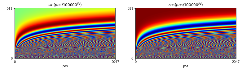
Figure 3. Time code for superimposition onto token embedding.
Output layer
The output from the final transformer block is the same size as the input to the first transformer block (\(seqlen \times d\)). On top of this we add a linear layer operating pointwise (i.e. an affine mapping in the \(d\) direction) and expanding to the \(vocab\_size\). In evaluation mode, we may only be interested in applying this final layer over a segment of the output tensor shown as \(seqlen'\times d\). In training \(seqlen' = seqlen\).
Finally, softmax is applied pointwise over the \(d\) dimension to produce a probability distribution over the vocabulary at each position.

Figure 4. Output layer for the transformer.

Figure 5. Showing the tensors in the output layer.
Training
Training is similar to the procedure used for the RNN. We fill the context window with token sequences and minimise the negative log likelihood of the same text shifted to the left by one position. With a context window of size 2048, as in GPT3, there is typically room for between 10 and 100 (tokenised) sentences. For GPT3, the batches contained 3.2M examples and there are 175B parameters that must be optimised in training. The compressed text corpus from which examples are drawn is 570Gb in size, amounting to around 400 billion tokens.
Evaluation
Evaluation in language generation is similar, but not identical, to the procedure used for RNNs. We start with a short tokenised text string in the context window, padded to fill the whole size of 2048. We then pass this through the transformer and sample from the distribution obtained at the position of the final token making up the prior text. The earlier outputs are ignored. Note that we only need to generate outputs up until the length of the tokenised text input since there is no need for the outputs beyond this. Next we concatenate the sampled token onto the end of the tokenised input text, re-run the transformer and sample the next token. This process repeats until the required number of tokens has been generated. The difference from the procedure we used for RNNs is that there we could continue generating new tokens indefinitely by passing the hidden state forwards at each time step. In the transformer, we re-run on the whole input each time, with a token string that gets progressively longer. When the context window is full, we can start to lose tokens from the start and continue to extend the generated text on what remains. When this happens, the memory of what went before, will be completely lost. In principle, an LSTM could retain memories for longer.
The GPT3 model has been demonstrated for news article generation. The following example is primed with the text in black (i.e. this is placed in the context window), and then novel text (shown in red) is generated by the transformer from this position:
Title: Star’s Tux Promise Draws Megyn Kelly’s Sarcasm
Subtitle: Joaquin Phoenix pledged to not change for each awards event
Article: A year ago, Joaquin Phoenix made headlines when he appeared on the red carpet at the Golden Globes wearing a tuxedo with a paper bag over his head that read, "I am a shape-shifter. I can't change the world. I can only change myself." It was a promise to not change to fit into the Hollywood mold: "I think that's a really special thing, to not change yourself. I think it's a really special thing to say, `This is what's inside of me, I'm proud of it, and I'm not going to be ashamed because of the way that someone else thinks I should be.'" Now, it's the Oscars, and Phoenix is at it again. But this time, his publicist is saying he'll be wearing a tux no matter what. Megyn Kelly was not impressed, and she let him have it on The Tonight Show. "You know, I feel like, I feel like you could have worn the tux," she says. "But you're saying you're a shape-shifter. I don't know if you can change your tux, but you can change your mind. You can change your mind. You can change your mind." Phoenix says he did, but it didn't stick "I was like, `Okay, I'm going to wear a tuxedo to this thing.' And then I thought, `I don't want to wear a tuxedo to this thing.'" Kelly goes on to encourage him to change his mind again, but Phoenix says it's too late: "I'm committed to wearing this."
Full transformer
In the original transformer paper (Veswani et al.), the transformer is divided into an encoder and a decoder. The model is intended for mapping from input text to an output text, where a representation for the input text in its entirety is constructed before starting on generating the output text. This works particularly well for machine translation, where the whole input needs to be read before attempting to produce a translation.
The overall architecture looks like this:
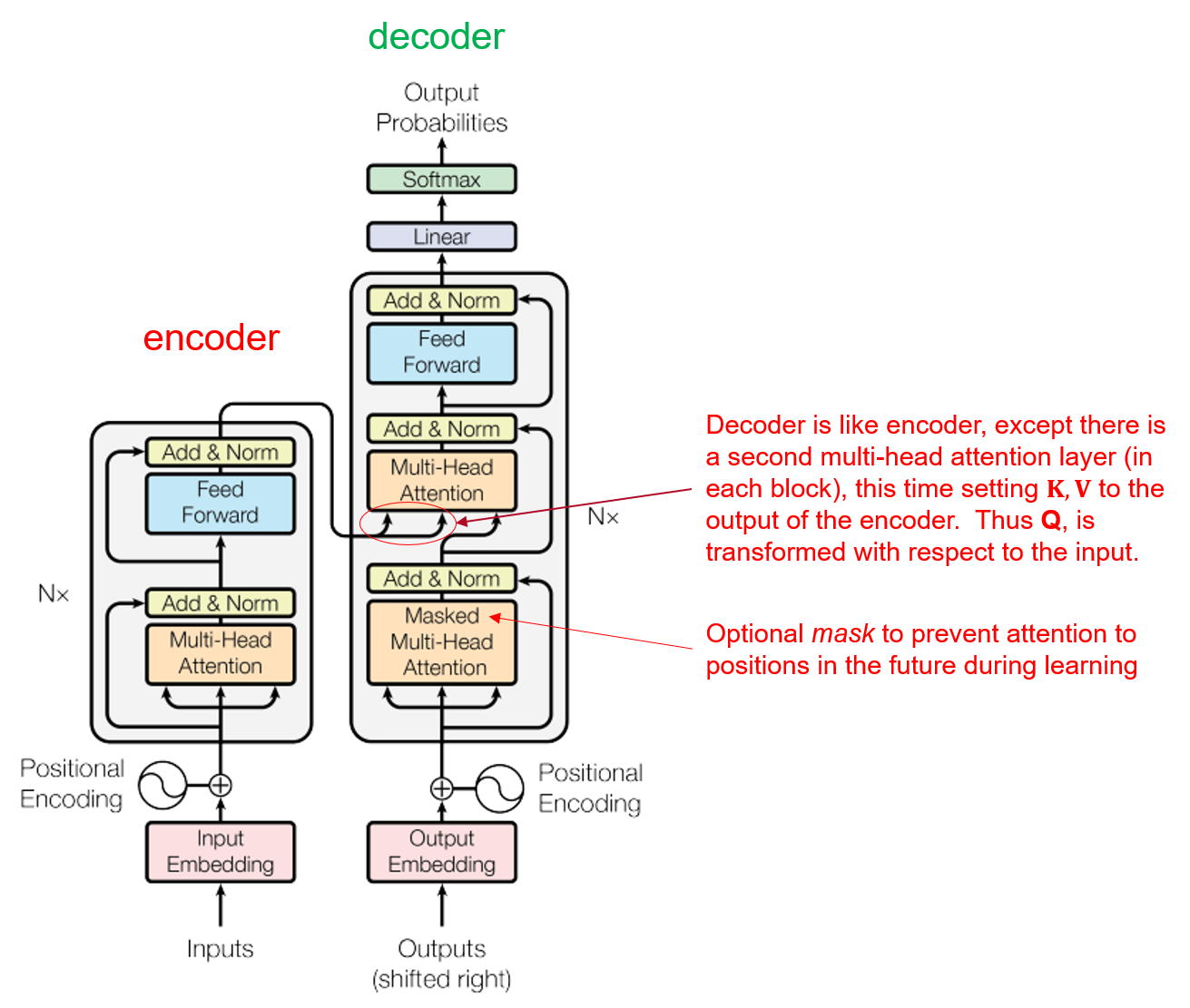
Figure 6. The full encoder-decoder transformer model.
The encoder and decoder are similar in design to the transformer model we have examined above. The encoder doesn't have the final linear layer (with softmax) and simply produces the output from the final transformer block. This output in its entirety becomes the representation of the source text from which the decoder will produce a translation.
The decoder has a second multi-head attention layer in each block. These layers are used as the entry point for the representation received from the encoder. The output from the encoder is used as the source of the keys \(K\) and values \(V\) input to the second attention layer in every block. The queries \(Q\) on the other hand flow up from within the decoder. In this way, the source text influences the decoder within every transformer block.
The final translation is obtained from the decoder by simply generating text in a similar fashion to the earlier language generator above. Rather than sampling from the output distribution at the position of the final input token, we can simply take the token with the maximum probability. This greedy strategy produces our output translation.
In detail, we first train the model with pairs of source and target texts in the different languages (e.g. English into French). The source text is input to the encoder, and the target text is input to the decoder shifted one place to the right and with a <start> token entered in the first position. This identifies the start of a target text in the first position. The loss is the negative log likelihood of the target text with an <end> token tacked on the end. The likelihoods are given by the probability distributions generated by the decoder and linear output layer (with softmax).
Having trained the model, we move into evaluation mode to produce translations of new source texts. The source text is input to the encoder and the output representation passed across to the decoder to be used as keys and values
by the second multi-head attention layer in each block. The decoder receives a single

Figure 7. Generating the first output token from a source text.
Select the maximum probability token from the decoder output distribution in the first position. In this case it is a token corresponding to the letter 'l'.
Next, repeat the process, except that the input is extended to two tokens by appending the 'l' token to the <start> token. Now read off the maximum probability token in the second position, ignoring the output in the first position. In this case, it is a token corresponding to the letter 'e'.

Figure 8. Generating the second output token from a source text.
This process repeats until the most probable output token is <end>.

Figure 9. Repeating the generation of tokens until the <end> token is the most probable.
Reading
Read the 2020 paper on GPT3 from Brown et al. at Open-AI [3]. Read sections 1, 2, 5, 6 and 8. Browse through section 3 to get a feel for the range of tasks that GPT3 can be used for (see for example 3.9.4 on news article generation).
References
[2] Radford, A. ‘Improving Language Understanding by Generative Pre-Training’, 2018.