Image segmentation
The semantic segmentation task is to label each and every pixel in a given image with the object class to which it belongs, including a catch-all class for the background. The examples below are from the Pascal VOC 2011 dataset. On the left are the original images and on the right are the ground-truth segmentations, where each pixel is colour-coded with the object class to which it belongs.

Figure 1. Illustrating the semantic segmentation of two natural images.
From Pascal VOC dataset.
Performance measurement
The performance of a method for semantic segmentation is normally measured using the so-called Jaccard index, which is a statistic for measuring the similarity between a pair of sets, \(A\) and \(B\).
The Jaccard index is defined as the size of the intersection over the size of the union of the two sets, expressed formally as:
The Jaccard Index is also referred to as Intersection over Union.
Applied to semantic segmentation, we ignore the background class (shown in black in the example above) and focus only on the labels associated with the objects of interest. For each label, we compute the Jaccard index of the set of pixels with that label in the segmentation with the set of pixels with this label in the ground-truth. The overall performance statistic is the mean of these indices over all object classes.
Often the object pixels will be represented by rectangles or arbitrary closed contours as shown below:

Figure 2. The Jaccard index is computed from a pair of sets. In this case the sets are represented by overlapping closed regions in 2D.
In general however, the pixels from a class may form two or more disjointed regions in the image and/or ground-truth.
Patch-wise classification
One approach to semantic segmentation is to simply train a classifier on small square patches surrounding each pixel, together with the class label assigned to the pixel. This is the approach adopted by Ning et al. [1].
The aim here was to segment microscope images of C. elegans embryos. C. elegans is a tiny worm that is barely visible to the human eye. The pixels of the images are to be segmented with five class labels: nucleus, nuclear membrane, cytoplasm, cell wall, and external medium. The embryo images are grey-scale (i.e. one channel) and vary in size, but are typically around \(300 \times 300\).
Note
The 50 images are taken from five videos of varying sizes (10 image frames per video). A size of \(300 \times 300\) is assumed below for simplicity.
Examples of embyo images together with segmentations are shown below. The second and third rows show the segmentation results using different ground-truths for training.
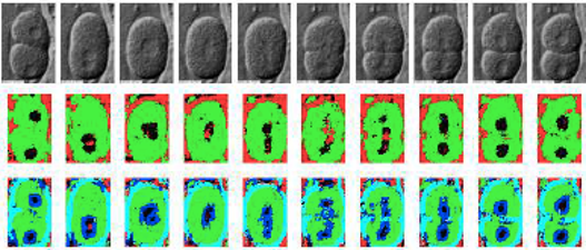
Figure 3. Two segmentations of C. elegans embryo images into five classes: nucleus, nuclear membrane, cytoplasm, cell wall and external medium.
From Ning et al. [1].
In experiments, Ning et al. extract patches around each pixel of size \(40 \times 40\). The patches are classified using a CNN with three convolution layers with no padding.

Figure 4. CNN for patchwise classification of pixels, giving a semantic segmentation.
CNN architecture taking in a 40x40 patch surrounding the pixel to be classified. The first stage is convolution with a 7x7 kernel into 6 feature maps. Second stage is 2x2 mean-pooling with a stride of 2. Third stage is convolution with a 6x6 kernel into 16 feature maps. This is followed by 2x2 mean-pooling, then another convolution with 6x6 kernel into 40 feature maps. Final stage is a fully connected layer from 40 into the five class confidences for the target pixel. The tanh activation function is used throughout and the convolutions are all without padding, meaning that the output from the final convolution consists of 40 1x1 feature maps.
The final convolutional layer outputs 40 feature maps each containing a single value. From just 50 training images, 190,440 \(40 \times 40\) patches are obtained, each associated with the label assigned to a centre pixel. Training uses the mean squared error loss function (see below).
The output is a set of maps of class confidences, illustrated below:

Figure 5. Illustrating the output confidence values for each of the five classes. Higher confidences are represented by lighter pixels.
From Ning et al., 2005.
The whole process can be made much more efficient by inputting a whole embryo image into the network at once. This is at the expense of a four-fold reduction in resolution of the final segmentation map due to the two pooling steps. However, it results in the same computation leading to each target pixel.

Figure 6. CNN for segmenting the whole image at once without breaking into patches.
The architecture of the network is the same as in Figure 4 up until the fully connected layer. The difference is that the whole 300x300 image is passed into the network instead of a single patch. This means that the tensors at each stage are much larger. The fully-connected layer (fcl) is replaced by a 1x1 convolution, which effectively replicates the fcl at each location, computing an affine function of the values across the 40 feature maps. The output is a 5x66x66 tensor providing class confidences over a 66x66 confidence map.
Mean Squared Error (MSE) loss function
Assume input \(\myvec{x}\), network output \(f(\myvec{x})\) and training data \(\{\myvec{x}^{(1)},\dots,\myvec{x}^{(m)}\}\), \(\{\myvec{y}^{(1)},\dots, \myvec{y}^{(m)}\}\) containing \(m\) examples. The Mean Squared Error loss is defined as:
For example, if we want the output \(\myvec{y} = f(\myvec{x})\) to be a probability distribution over class labels, we provide one-hot vectors as the ground-truth. For example, the class cytoplasm is represented by the ground-truth output vector \((0,0,1,0,0)\). This is ideally what we would like the network to output when cytoplasm is the true class. This is an alternative to negative log likelihood loss (cross-entropy loss).
The one-hot encoding for elements from an ordered set (e.g. class labels) is defined in the section on Text classification.
Encoder-decoder and U-Net architecture
A second way to produce a semantic segmentation is using an encoder-decoder architecture, which we depict as follows:

Figure 7. Encoder-decoder architecture for semantic segmentation.
The images are from the Pascal VOC dataset .
The idea is that the encoder produces a compact encoding of the input image within an embedding layer and the decoder expands this encoding into a semantic segmentation. The encoder and decoder will typically be multilayer CNNs. Conceptually, the encoding is a compressed representation of the input that succinctly captures patterns in the image structure from which the decoder can construct the required semantic segmentation. By forcing the information flow through the constriction, we encourage the emergence of common patterns that encode the image. This is the same intuition that underlies the semantic embedding of the words in a piece of text that we will be examining in the section on Text classification.
A powerful extension of this idea is the U-Net architecture, which is essentially an encoder-decoder network with shortcuts that link successive layers of the encoder to the corresponding layers of the decoder. This is naturally represented by depicting the network as a 'U' shape - hence the name. The original idea for the U-Net architecture for semantic segmentation is due to Ronnerberger et al. [2].
We will look at a newer version used within a system for diagnosis and referral in retinal disease due to Faux et al. [3].
The images are obtained from a technique known as Optimal coherence tomography (OCT) and are each 3D scans of the tissue around the macular in the back of the eye. Each image is of size \(488 \times 512 \times 128\) slices. Given an OCT image, the aim of the system is to produce one of four referal options: urgent, semi-urgent, routine or observation only; and 10 diagnostic options (e.g. geographic atrophy, normal). The system works in two stages. The first stage produces a semantic segmentation of the 3D OCT image. The second stage is a pair of classifiers generating probability distributions for the referall options and for the diagnostic options. The two stages are illustrated in the following diagram:
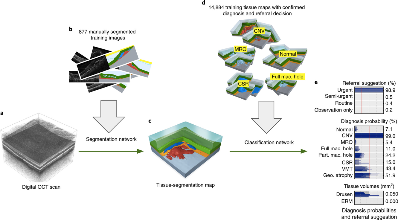
Figure 8. The classifier works in two stages. The first stage produces a tissue (semantic) segmentation map from the 3D OCT scan. This is trained using a corpus of manually segmented images and uses a U-net architecture. The second stage is a CNN-based classifier of the tissue maps into referral and diagnosis confidence/probability values. This stage is trained using tissue segmentations with confirmed diagnosis and referral decisions from patient records.
A 3D OCT scan is depicted on the left, mapping into a 3D tissue segmentation map in the middle, which maps into referrall and diagnosis values on the right. The training data is shown above the two mappings in each stage.
From Faux et al. [3].
The two parts of the system were trained separately. Training the U-Net made use of 877 manually segmented training images, and training the classifier made use of 14,884 semantic segmentations (tissue maps) with the confirmed diagnosis and referral labels (decisions).
The U-Net architecture used for semantic segmentation is shown below:
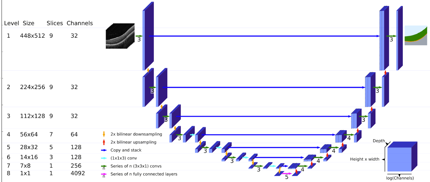
Figure 9. The U-Net architecture used for producing tissue segmentation maps from OCT scans.
The architecture is similar to the original U-Net model. The input on the top-left consists of 9 consecutive slices from the OCT scan, each of size 448x512. This passes through three convolutions with 32 channels (feature maps). The progressive bilinear downsampling through 8 levels, ends with 1 slice of size 1x1 and 4092 channels (bottom middle). This 4092 vector passes through 5 fully-connected layers before being progressively upsampled through 8 corresponding layers to produce a single output slice of the tissue segmentation map at the top-right. Cross-links feed the final feature maps at each level on the downside (left) across to be concatanated with the initial feature maps at each level of the upside (right).
From Faux et al. [3].
The U-Net is configured to produce 2D segmentations corresponding to single 2D slices of the OCT scan. The input to the U-Net is a set of nine slices, four either side of the target slice. Thus, the U-Net runs multiple times to build up a 3D segmentation map, slice by slice, from a 3D OCT scan. In detail, the input is a 3D tensor of size \(448 \times 512 \times 9\). At the first level, the input tensor goes into a sequence of three convolutional layers, each performing 3D convolutions into 32 channels with \(3 \times 3 \times 1\) kernels. Note that the first layer operates directly on the section of the OCT scan. As usual, the second and third layers sum convolutions over the 32 channels from the previous layer - this can be thought of as performing a 4D convolution over all 32 channels.
The result from level one is a 4D activation map of size \(448 \times 512 \times 9 \times 32\). The spatial dimensions are now downsampled by a factor of two using bilinear interpolation, giving an activation map of size \(224 \times 256 \times 9 \times 32\). The three convolutional layers are repeated and the result is again downsampled by a factor of two giving an activation map of size \(112 \times 128 \times 9 \times 32\). These are now downsampled again giving an activation map of size size \(56 \times 64 \times 9 \times 32\). Three more convolutions are performed, this time into 64 channels. This is followed by a convolutional layer with \(1 \times 1 \times 3\) kernel size to combine data across the slice dimension, generating an activation map of size \(56 \times 64 \times 7 \times 64\). Notice the reduction in the size of the slice dimension due to not using padding in this final convolutional layer. The same process is repeated in the next three levels, ending up with an activiation map of size \(7 \times 8 \times 1 \times 128\). This is downsampled once more, flattened and passed through five fully connected layers.
The result now travels back up through the levels, with bilinear upsampling replacing downsampling and analogous convolutional layers. The final output has the same spatial size as the input image and depth equal to the number of classes. Taking the maximum over the depth dimension gives the label at each spatial location.
So far we have ignored the cross-links. These simply take the final activation maps at each level on the encoder side and concatenate with the input activation maps at the same level on the decoder side. The idea is that detailed feature maps obtained during encoding are available directly at the decoder stage, where they are combined with contextual information that passes from higher levels. Conceptually, you can think of the class probabilities assigned to each pixel as being influenced by a combination of information from different spatial scales, ranging from the evidence in the immediate vicinity of the pixel (from the cross-link) to global aspects of the image (from the chain leading up from the embedding at the base of the 'U').
The classification stage is a CNN classifier applied directly to a one-hot encoding of the segmentation map. The segmentation map is subsampled from \(448 \times 512 \times 128\) to \(300 \times 350 \times 43\).
Reading
You should read the Nature paper that describes this system (Faux et al. [3]). We will discuss the paper in the webinar next week. The main paper gives a lot of background and outlines the way in which the system works. The technical details are contained within a methods section at the end and there are many additional figures (including the U-Net architecture) and videos in the supplementary material.
Bilinear interpolation
An important part of the segmentation network is the downsampling and upsampling using bilinear interpolation. The definition of bilinear interpolation is as follows:
Given \(z_{ij}\in \mathbb{R}\), defined over a 2D rectangular grid of points \({(x_i ,y_j)}\), we seek to derive a new grid of points at higher or lower resolution. For some point \((x,y)\) in the new grid, the bilinear interpolated value \(z\) at this location is given by linearly interpolating at the \(x\) intercept between the values at the grid points above and below the new point, to give \(z'\) and \(z''\), and then linearly interpolating between \(z'\) and \(z''\) at the \(y\) intercept to give \(z\).

Figure 10.Bilinear interpolation of the function at a given point works with a grid of values. First the function is approximated between adjacent horizontal grid points on the grid lines above and below the target point by linear interpolation, z' and z''. Then the function value z at the target point is approximated by linear interpolation between the values z' and z''.
A 4x4 grid of known points is shown. A target point (x,y) within the inner grid square is labelled with the value z, which is to be found. The grid line at the bottom of the inner square shows the value z' obtained at horizontal coordinate position x and the grid line at the top of the inner square shows the value z'' also at x. A vertical dotted line through z', z, and z'' represents the final linear interpolation that gives the required value of z.
Note that the bilinear interpolation in the U-Net enters into the gradient function since it changes the activation maps.
In downsampling of images, it may be necessary to smooth the image first using Gaussian convolution to prevent aliasing effects that arise from high spatial frequency content in the image. It seems probable that this wasn't done here.