Linear classifier
In this section we look at the linear classifier. This will help to motivate the key ideas in a deep feedforward network.
Classifying iris flowers
The idea of a linear classifier goes back to before the field of AI began. We start with the often used example of Iris classification, where the problem is to classify iris flowers into one of three species: Iris setosa, Iris versicolor and Iris virginica.
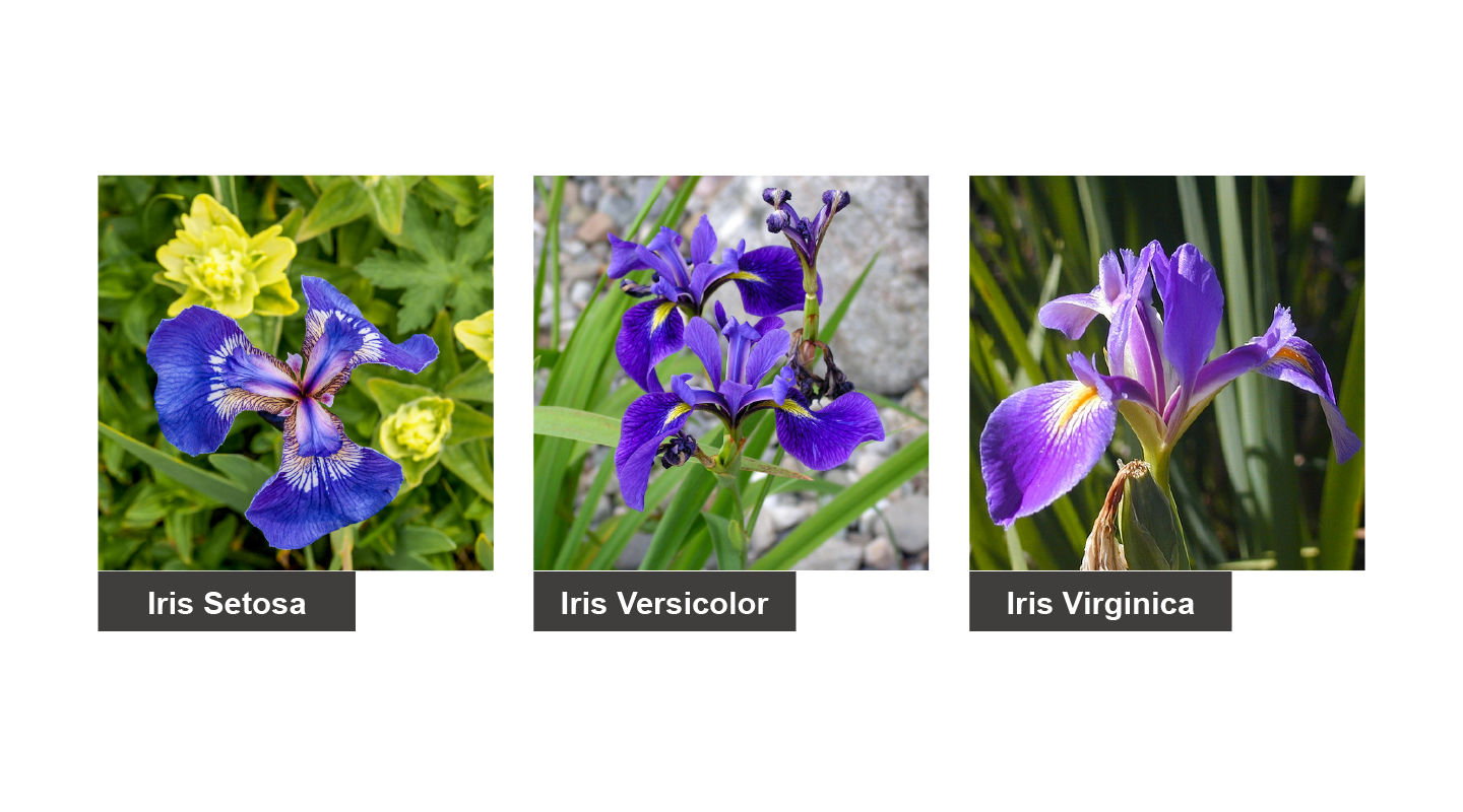
Figure 1. Three classes corresponding to three species of Iris flowers.
The classification is based on four measurements: the length and width of sepals and petals, as shown below:
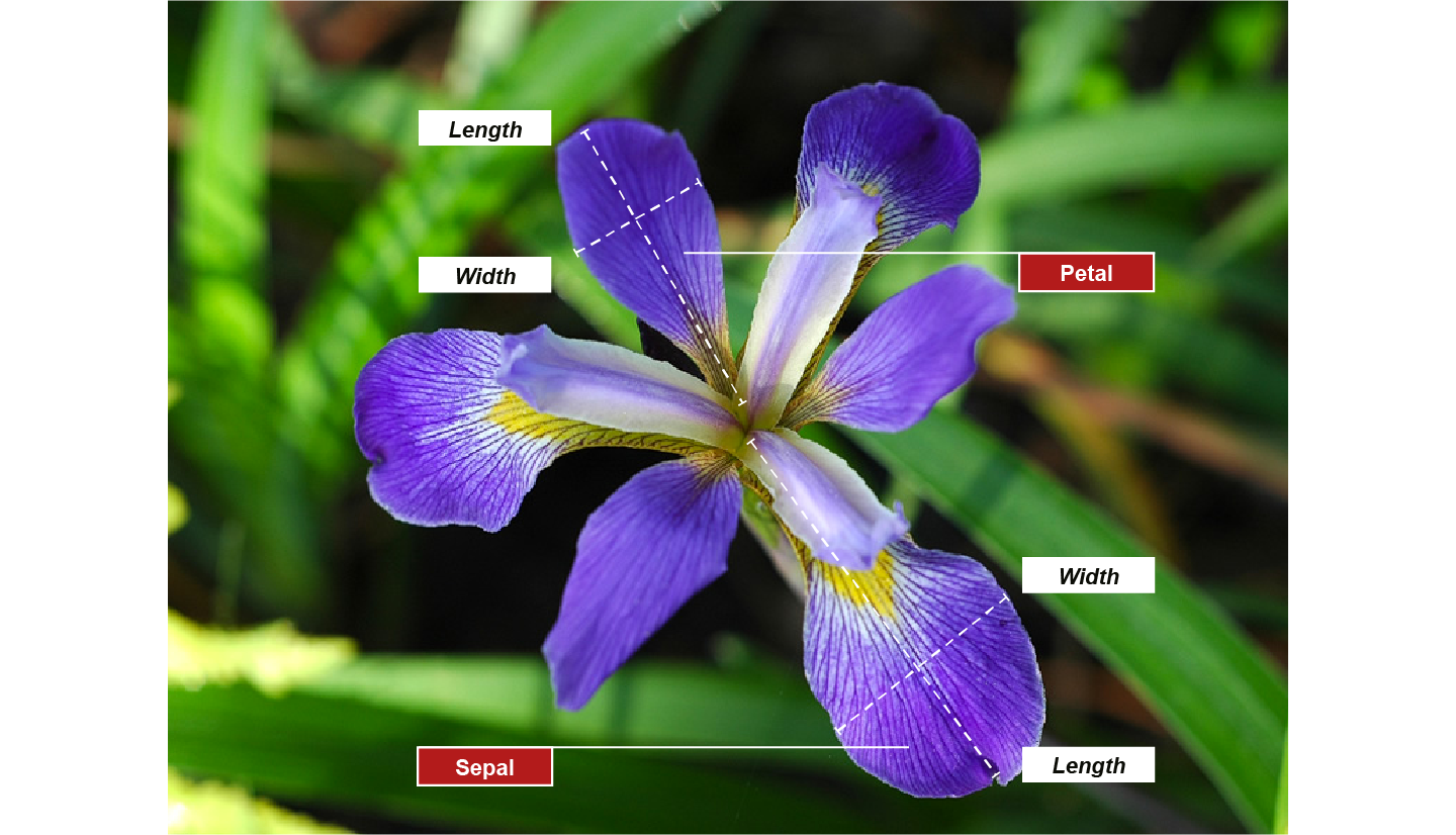
Figure 2. In the Iris dataset, a flower is represented by four measurements.
The dataset consists of 120 iris flowers, with four measurements each, as shown in this extract of the table:
| Dataset order | Sepal length | Sepal width | Petal length | Petal width | Species |
|---|---|---|---|---|---|
| 1 | 5.1 | 3.5 | 1.4 | 0.2 | l. setosa |
| 2 | 4.9 | 3.0 | 1.4 | 0.2 | l. setosa |
| 3 | 4.7 | 3.2 | 1.3 | 0.2 | l. setosa |
| 4 | 4.6 | 3.1 | 1.5 | 0.2 | l. setosa |
| 5 | 5.0 | 3.6 | 1.4 | 0.3 | l. setosa |
| 6 | 5.4 | 3.9 | 1.7 | 0.4 | l. setosa |
All measurements are in centimetres. The class labels are encoded as integers: 0 for Iris setosa, 1 for Iris versicolor, and 2 for Iris virginica. You can read about the dataset at https://en.wikipedia.org/wiki/Iris_flower_data_set.
To understand more about the distribution of the data, consider the following scatterplots comparing different pairs of measurements for all flowers. For example, the scatterplot in the second column of the first row compares sepal width on the horizontal axis with sepal length on the vertical axis. The different types of iris are colour-coded as shown.

Figure 3.Pairwise scatterplots of petal and sepal measurements. Licensed under the Creative Commons Attribution 4.0 International license.
12 scatterplots showing each of the four measurements on the horizontal axis plotted against the three other measurements on the vertical axis. Six of the scatterplots are transpositions of the other six, exchanging horizontal and vertical axes. Individual flowers are colour coded to denote one of the three classes. The scatterplots demonstrate that the examples of versicolor and virginica flowers cannot be separated by a line for any pair of measurements. By contrast, the examples of setosa flowers can be separated from the other two with any pair of measurements.
Image classification
Classification of images into different classes is a major topic in AI with many potential applications. Given the following image, we might seek to classify it into one of three classes: car, bike or truck. Or we might seek to classify it into an indoor or outdoor scene, or to whether it is raining, sunny or cloudy.

Figure 4. This image could be classified in many different ways.
A particularly challenging classification task is to identify the face in an image from millions of possibilities, as here:

Figure 5. Facial identity recognition is a standard image classification task.
In general, these are hard problems because of:
- variations in viewpoint and lighting
- intra-category variation
- shape deformation
- distraction from other objects and scene background.

Figure 6. The following images of cats are all very different from one another for a variety of reasons.
For faces, there is also the problem of changing appearance with age and obscuring objects such as glasses.

Figure 7. People change their appearance with age and apparel.
The research community makes use of standard datasets as benchmarks against which to compare different classification methods. These include the MNIST dataset consisting of 70,000 28x28 images of handwritten digits, each classified with one of ten class labels corresponding to the digits from 0-9, as in the examples below:
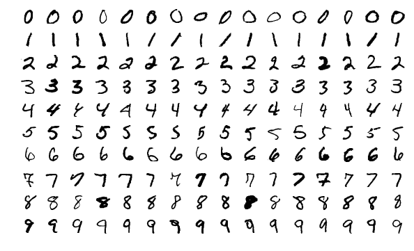
Figure 8. Examples from the MNIST dataset of 70,000 28x28 images of handwritten digits. CC BY-SA 4.0
The CIFAR-10 dataset contains 6000 32x32 RGB images for each of 10 object categories.
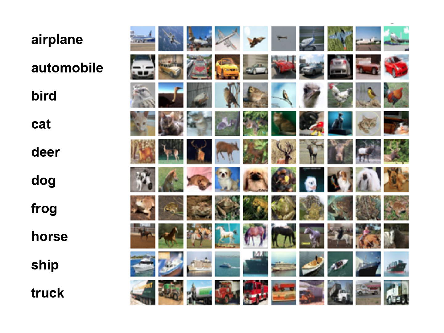
Figure 9. Examples from the CIFAR-10 dataset. From https://www.cs.toronto.edu/~kriz/cifar.html
The CIFAR-100 dataset contains 600 32x32 RGB images for each of 100 object categories.
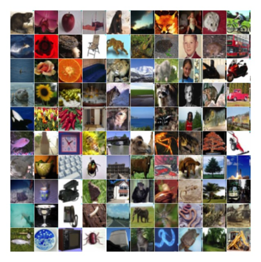
Figure 10. Examples from the CIFAR-100 dataset. From https://www.cs.toronto.edu/~kriz/cifar.htm
Linear classifier for 2-D data and two classes
Returning to the classification of iris flowers, suppose we choose two measures: petal length and petal width. We then attempt to discriminate between images of Iris setosa and images of Iris versicolor. A linear classifier would attempt to separate instances of the two classes by a straight line. The following scatter plot shows the dataset of iris flowers, each represented by \(2D\) vectors \((x_1,x_2)\) corresponding to petal length and petal width. Here it is possible to draw a straight line that separates Iris setosa and Iris versicolor from one another – we say they are linearly separable.
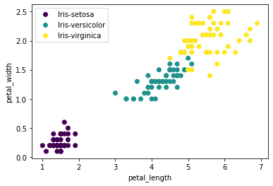
Figure 11. Scatterplot of petal length against petal width for the Iris dataset.
Scatterplot showing that the examples of Iris setosa and Iris versicolor in the Iris dataset are easily separated from one another by a straight line.
The equation of a line has the form:
where \(w_1, w_2\) determine the orientation of the line, and \(b\) determines the distance from the line to the origin.
If you substitute a datapoint \((𝑥_1,𝑥_2)\) into the left-hand-side of the line equation, the value obtained will be positive for points on one side of the line and negative on the other. Thus, we have an easy way to determine whether a given flower is Iris setosa or Iris versicolor. Denoting Iris setosa by the label 0 and Iris versicolor by the label 1, we have:
Linear classifier for n-D data and two classes
All of this readily generalises to n-dimensional data, where the equivalent of the line is a hyperplane, given by:
We can write this succinctly using a dot product as \(\myvec{w}\cdot\myvec{x}+b=0\).
Using matrix notation and expressing as column vectors \(\myvec{x}=[x_1\dots x_n]^T\) and \(\myvec{w}=[w_1 \dots w_n]^T\) we can also write this as a matrix product \(\myvec{w}^T \myvec{x}+b=0\).
Just as for a line, a hyperplane divides the \(nD\) space into two parts. Substituting a data point into the left-hand-side of the equation above gives a positive value on one side of the hyperplane and negative on the other. Thus, in terms of the dot product, we have:
Note that the vector \(\myvec{w}\) is perpendicular to the hyperplane. The perpendicular distance of the hyperplane to the origin is given by \(\frac{b}{||\myvec{w}||}\). The perpendicular distance \(d\) of a point \(\myvec{x}\) to the hyperplane is given by \(d=\frac{\myvec{w}.\myvec{x}+ b}{||\myvec{w}||}\), where \(d\) is positive on the side of the hyperplane in the direction of \(\myvec{w}\) and negative on the opposite side.
More explanation on the geometry
A plane or a hyperplane is generally defined by a normal vector which, by definition, is perpendicular to the hyperplane and determines the inclination or orientation of the hyperplane in the space. Since there are infinitely many planes that can be perpendicular to the normal vector, we also need a single point on the hyperplane to be able to uniquely define it.
Let’s call the normal vector \(\myvec{w}\) and the point on the hyperplane \(\myvec{x_0}\) . Now let’s assume another arbitrary point \(\myvec{x}\) on the hyperplane. Since \(\myvec{x}\)and \(\myvec{x_0}\) are both on the hyperplane, the vector \(\myvec{x}−\myvec{x_0}\) is also on the hyperplane. We know from the definition that all vectors on the hyperplane must be perpendicular to the normal vector. Therefore, all vectors of the form \(\myvec{x}−\myvec{x_0}\) must be perpendicular to the hyperplane. In mathematical terms, the dot-product of \(\myvec{x}−\myvec{x_0}\) and the normal vector \(\myvec{w}\) must be zero. This gives us the plane equation:
We can expand this to get:
Now let \(b=−\myvec{w}\cdot\myvec{x_0}\) . This gives you the plane equation above: \(\myvec{w}\cdot\myvec{x}+b=0\) .
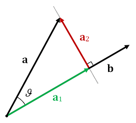
As background for understanding the computation of distance from the origin, you need to know about vector projection. To get the projection length of a vector \(\myvec{a}\) onto a straight line parallel to another vector \(\myvec{b}\) , we use the following equation:
where \(\hat{\myvec{b}}\) is the unit vector \(\frac{\myvec{b}}{∥\myvec{b}∥}\) and \(a_1\) is the length of the vector \(\myvec{a_1}\) .
To derive the distance equations, it’s easier to work with the following formulation of the hyperplane (derived above):
The term \(b=−\myvec{w}\cdot\myvec{x_0}\) can be used to find the projection of the vector connecting the origin and the point \(\myvec{x_0}\) onto a straight line parallel to the normal vector \(\myvec{w}\) . If we normalise this by the length of the normal vector, we get the length of the projection which is technically the closest distance from the origin to the hyperplane:
Note that the absolute value in the numerator is needed because dot-product can be positive or negative depending on the angle between the vectors.
We can use the projection idea to derive the distance from an arbitrary point. Assume an arbitrary point \(\myvec{x}\) in the space. The vector \(\myvec{x}−\myvec{x_0}\) is the vector connecting \(\myvec{x_0}\) on the hyperplane and the point \(\myvec{x}\) . The projection length of this vector along the straight line parallel to the normal vector is:
For the classification purposes explained in the notes, we can drop the absolute value from the numerator to be able to use the sign to find out on which side of the plane a given point resides. This is related to the angle the vector \(\myvec{x}−\myvec{x_0}\) makes with the normal vector \(\myvec{w}\) .
Linear multiclass classifier
Suppose now we have K classes (\(K \ge 2\)). We can build a multi-class classifier by associating a separate hyperplane with each of the \(K\) classes \(\{\myvec{w}_c.\myvec{x}+b_c=0 \}_{1 \leq c \leq K}\). The idea is that each hyperplane separates the associated class from the remaining classes. The figure below illustrates this idea for four classes and \(2D\) datapoints. The clouds represent clusters of datapoints from a single class.

Figure 12. Examples of four classes represented by the four data clouds. Each cloud of data can be separated from the other three by a straight line.
The distance from the associated hyperplane in the positive direction can be regarded as a measure of confidence in this class being the correct label. Assuming \(\myvec{w}_c\) is already scaled to be a unit vector, the confidence values are given by:
We simply choose the class with the highest confidence value: \(\underset{c}{\operatorname{argmax}(z_c)}\)
Defining a probability distribution over class labels
From our confidence values, we can compute a probability distribution using the softmax function:
Softmax takes the set of confidence values, which may be negative, and returns corresponding values between \([0,1]\) which sum to one, as required for a probability distribution. The exponential function in the numerator of softmax is a monotonically increasing function with positive output.

Figure 13. The exponential function is positive and monotonically increasing.
Thus, the higher the confidence value (even if negative) the higher the probability. The denominator ensures that the values sum to one.
For example, suppose the confidence values for 3 classes are given by \((2.1, 1.2, -1.5)\). The probability distribution computed by softmax will be \((0.70, 0.28, 0.002)\).