Multilayer networks
Introduction
Our multiclass classifier computes a set of confidence values using affine equations of the form \(z_c = {\myvec{w}_c}\cdot\myvec{x} + b_c\).
We can express this as a single affine matrix equation generating a column vector of outputs (confidence values) \(\myvec{z} = [z_1 \cdots z_K]^T\) as follows:
where \(\myvec{b} = [b_1 \cdots b_K]^T\) and the rows of \(W\) are the weight vectors \(\myvec{w}_c\).
We generate a probability distribution from \(\myvec{z}\) using softmax.
Consider the following two-class classification task for 2-D feature vectors:

Figure 1. Examples from two classes (red and blue) are grouped into four clusters. The examples from the two classes are not linearly separable.
We can't configure a linear classification to do this because there is no line that separates the two classes. Of course, it is easy to see how we might resolve this problem by simply treating the individual clusters as separate classes and then adding additional machinery to select from these in making the classification we require. It turns out we can do this by feeding the output from the affine function into a second affine function.
We might be tempted to do the following:
But this reduces to:
which is again a simple affine function of the form:
where \(\mymat{W}_3 = \mymat{W}_2 \mymat{W}_1\) and \(\myvec{b}_3 = \mymat{W}_2 \myvec{b}_1+ \myvec{b}_2\)
Instead, we introduce a non-linear function between the two affine functions in order to accentuate the highest values from \(f_1\). In the neural network literature, this non-linearity is known as an activation function. We will see that adding yet more layers often improves performance further. Each layer is separated by an activation function. Three of the most common activation functions are introduced below.
The logistic function
The logistic function drives outputs towards one for positive inputs and towards zero for negative inputs.

Figure 2. Graph of the logistic function.
We use this to emphasise high confidence values, driving low values towards zero.
The logistic function is often referred to as the sigmoid function because of the 'S' shape.
The hyperbolic tangent (tanh) function
The hyperbolic tangent function, or tanh for short, squashes the input into the interval \((-1, 1)\), driving positive inputs towards 1 and negative inputs towards -1.

Figure 3. Graph of the hyperbolic tangent function.
The Rectified Linear Unit (ReLU) function
The rectified linear unit function, or ReLU for short, simply passes through positive inputs unchanged and outputs zero for negative inputs:

Figure 4. Graph of the Rectified Linear Unit function.
We'll see uses for all three activation functions during the module.
Terminology
The kind of multilayer network introduced above is normally referred to as a Multilayer Perceptron (MLP). The affine layers are referred to as Linear layers in PyTorch and Tensorflow, and Dense layers in Keras. They are also often referred to as fully-connected layers because every scalar value in the output from the layer is a function of every scalar value in the input to the layer. We will abbreviate fully-connected layer to fcl in network diagrams.
Training and testing
For a chosen dataset and classifier architecture, we divide the dataset into two parts: the first part for training and the second part for testing. We define a measure of performance which we call the loss function. The idea is to find values for the weights and bias values of the classifier that minimise the loss function computed on the training data. We then apply the resulting classifier to the test data to obtain a final measure of performance. It is important not to use the test data in any way during training.
Unfortunately, using this procedure, we won’t know how well we’ve generalised from the training data until it's too late and we have what may be a poor test result. In particular, the classifier may have over-fitted the training data in the sense that it produces a low loss (on the training data) but doesn’t generalise well to new data. The usual way around this is to further split the training data into two. The first part (confusingly also referred to as the training data) is used to minimise the loss function, and the second part (validation set) is used to check that the training has produced a good generalisation from the training data. We can explore a range of hyper-parameters (meta-parameters) and architectures to see what works best. After multiple rounds of training and evaluation on the validation set, the network is applied to the test data to produce a final measure of performance.
For the multiclass, multidimensional classifier introduced above, we must estimate the optimal values for the parameters associated with each of the \(K\) hyperplanes: \(\{(\myvec{w}_c , b_c) \}_{1 \leq c \leq K}\) in each layer.
Maximum likelihood loss function
We focus on classifiers for which the output is a probability distribution over class labels.
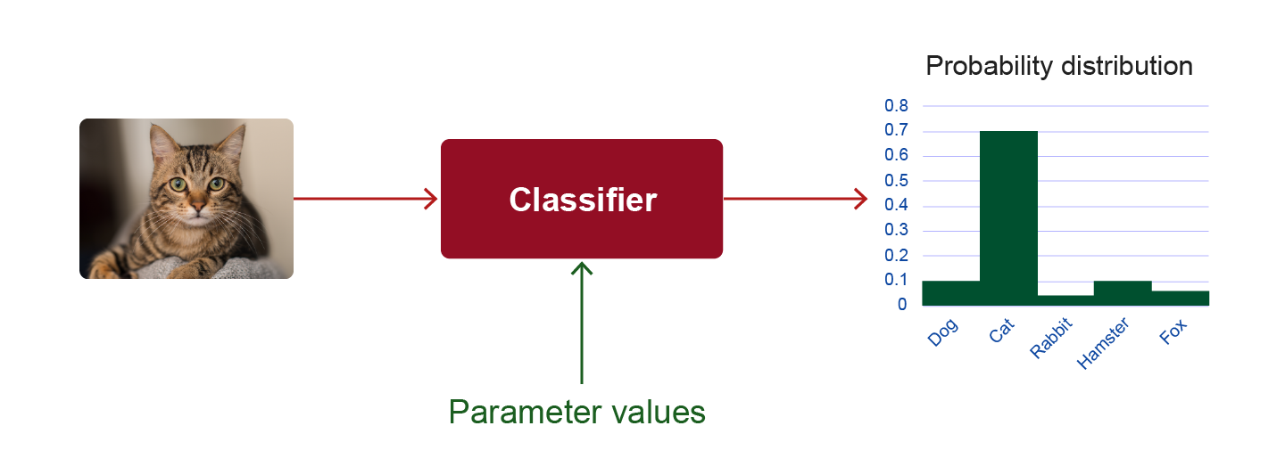
Figure 5. Classifier pipeline from an image to a probability distribution over the possible classes. The classifier is configured with a set of values for its parameters (weights and bias values).
For an input \(\myvec{x} \in \R^n\) let the probability from our classifier for a given class label \(y \in \{1,\dots ,K \}\) and model parameters \(\boldsymbol{\theta}\) be \(p(y|\myvec{x};\boldsymbol{\theta})\). Thus, \(p(.|\myvec{x};\boldsymbol{\theta})\) is a categorical probability distribution (i.e. a multinomial distribution with one draw).
Given training data \(\{\myvec{x}^{(1)}, \myvec{x}^{(2)}, \dots,\myvec{x}^{(m)}\}, \{y^{(1)},y^{(2)},\dots,y^{(m)}\}\) containing \(m\) labelled examples, the joint probability of these outputs given these inputs is:
We think of this as a function of \(\boldsymbol\theta\) since the training data is fixed, and we are interested in maximising the joint probability over \(\boldsymbol\theta\). Thus, we refer to this as a likelihood function since it can't be considered to be a probability density function, which would have to have unit area.
In training the classifier, we need to maximise the likelihood function to find the maximum likelihood solution, denoted by \(\boldsymbol\theta_{ML}\).
Before doing this, we avoid the product by taking the log of the likelihood, which enables us to rewrite the product as a sum (as in \(log(ab)=log(a)+log(b)\)).
Note that the \(\log\) function is monotonically increasing (i.e. \(x \ge y \implies \log(x) \ge \log(y)\)).

Figure 6. Graph of the (natural) log function.
Consequently, taking the log of the joint likelihood doesn't change the optimal value \(\boldsymbol\theta_{ML}\) that we seek.
We finish by negating the log likelihood to turn the maximisation into a minimisation:
The term we are minimising in this final equation is known as the negative log likelihood loss function or NLL for short. It is equivalent to the so-called cross entropy loss function.
Note: in PyTorch, NLL takes log probability as input, whereas cross-entropy loss takes raw confidence values.
Stochastic gradient descent (SDG)
To find the maximum likelihood solution \(\boldsymbol\theta_{ML}\), we use gradient descent on the loss function. Instead of doing this with a loss computed from all of the training data, we break the training dataset down into fixed sized chunks (minibatches) and perform gradient descent sequentially over each one in turn, each time starting with the previous estimate. The size of minibatches depends on the size of the problem and is often determined by the amount of data that will fit into a GPU.
Due to the small size of minibatches, there is some stochasticity (randomness) in the gradient descent (hence the name). This can help in generalisation.
After all examples from the training dataset have been used once, this marks the end of an epoch. The same procedure continues until a fixed number of epochs is reached or until the loss is no longer decreasing.
The input to the gradient descent is therefore a whole minibatch of data that is propagated jointly through the classifier to deliver a combined loss at the end. To build the computational graph required for backpropagation, we could iterate through the data elements in the minibatch one by one in order to compute the loss function on the set of outputs; remember that the loss function is computed on the outputs from the whole minibatch of data. It is more efficient however to perform the layerwise computations together, computing the first layer on the whole minibatch before moving on to the second layer and so on. To do this, we concatenate the minibatch into a single tensor.
Applying multilayer networks to MNIST
In this section, we build classifiers for the MNIST dataset. We will compare classifiers with one and two fully connected layers. The architectures of the two classifiers are illustrated as follows:

Figure 7. Classifiers with one full connected layer (left) and two fully connected layers (right).
The 1-layer pipeline on the left starts with an MNIST 28x28 grey-level (i.e. one channel) input image. This is flattened into a vector of size 784, passed through a fully-connected layer to a vector of size 10, and then through softmax to output a probability distribution of size 10. The 2-layer pipeline is similar, except that the first fully-connected layer outputs a vector of size 300, which passes through a sigmoid function before passing through a second fully-connected layer to a vector of size 10, and finally the softmax function.
The size of the tensor at each stage is shown in red. Note that we are showing the tensor sizes for a single input passing through the network rather than a minibatch of inputs. In PyTorch, the actual input size will be \(N \times 1 \times 28 \times 28\), where \(N\) is the number of samples in the minibatch.
The following graph shows the reduction in the loss over 200 epochs of stochastic gradient descent on the two classifiers. The classification accuracies are 92.6% and 97.8% respectively. As expected, the accuracy increases with the move from one to two layers.

Figure 8. Graph of the loss over 200 epochs of SGD for a 1-layer network (red) and 2-layer network (green).
A graph plotting the mean loss on the training data after each epoch for the 1-layer and 2-layer networks shown in Figure 7. The 1-layer network starts out with lower loss but immediately levels out. It is rapidly overtaken by the 2-layer network, for which the loss continues to decrease over 200 epochs.
Momentum in gradient descent
Gradient descent updates \(\boldsymbol\theta\) according to the gradient of the loss at its current value:
Several variations of gradient descent are motivated by thinking of \(\boldsymbol\theta\) as having momentum. Thus, the movement of \(\boldsymbol\theta\) through the parameter space is interpreted as a body in motion, with velocity \(\myvec{v}\). On each iteration it slows down a bit and gets nudged in the direction of the negative gradient (the direction of fastest decrease in \(f(\boldsymbol\theta)\) ).
The update to \(\boldsymbol\theta\) on each iteration is now:
Nestorov momentum is a slight variation on this. The gradient is evaluated after the current velocity is applied, thus:
Reading
To set the scene for what is to come in the module, and to look at the wider implications of deep learning and AI in general, read the 2019 paper by Eric Topol on the application of AI to medicine [1]. Topol is a clinician and has an interesting vision for the future of medicine in the light of progress in AI.