Measuring classifier performance
Confusion matrix
A simple and informative way of setting out the performance of a multiclass classifier is with a confusion matrix that sets out the number of correct predictions and the number of incorrect predictions (confusions) as a matrix such as this:
| Predicted class | ||||
|---|---|---|---|---|
| Car | Bicycle | Truck | ||
| Actual class | Car | 8 | 2 | 1 |
| Bicycle | 1 | 7 | 2 | |
| Truck | 2 | 0 | 12 | |
In this example, eight cars were predicted correctly and two cars were incorrectly predicted to be bicycles.
Accuracy
From the confusion matrix we can compute accuracy, the proportion of correct predictions and error rate, the proportion of incorrect predictions. Note that:
From the confusion matrix above we have:
Special case: binary classification
In the special case of binary classification (two classes), we are often most interested in one of the two classes. For example, for a classifier looking for faulty widgets on a production line, we are particularly interested in performance with respect to the faulty widgets.
To emphasise the relative importance of the two classes, we normally refer to the class we are interested in as the positive class and the other one as the negative class. The different outcomes corresponding to each cell in the confusion matrix are then referred to as indicated below:
| Predicted class | |||
|---|---|---|---|
| Positive | Negative | ||
| Actual class | Positive | TP = #(true positives) | FN = #(false negatives) |
| Negative | FP = #(false positives) | TN = #(true negatives) | |
Two ways of measuring the performance of binary classifiers are widely used.
True positive rate and false positive rate
The true positive rate (TPR) is the proportion of actual positives that are correctly predicted. In the example of faulty widgets, it is the proportion of faulty widgets that are correctly identified. The false positive rate (FPR) is the proportion of actual negatives that are predicted as positive. We could consider this to be the false alarm rate. In looking for faulty widgets, it is the proportion of perfect widgets (negatives) that are incorrectly classified as faulty.
The true positive rate is also known as the sensitivity.
There is a trade-off between the two measures TPR and FPR that depends on how strict we are in classifying things into the positive class. In classification, we have simply taken the category with the highest probability, which for binary classification means the category with probability greater than 0.5 (if the probabilities are equal we can choose either). Instead of doing this, we can set a higher threshold to be classified as positive, demanding greater confidence before assigning to this category. This recognises the implications of getting it wrong and enables us to strike a balance between TPR and FPR. We can reduce the number of false alarms (FPR) by increasing the threshold (a good thing), but at the cost of missing more of the positives and thereby reducing TPR (a bad thing). We can visualise this trade-off by varying the threshold and plotting TPR against FPR as a curve, as illustrated below. This is known as a Receiver Operating Characteristic (ROC) curve.

Figure 1. ROC curve.
ROC curve (in red) plotting TPR against FPR. ROC curve in green is for a baseline classifier that outputs random confidence values.
This ROC plot shows the performance (in green) of a baseline classifier that simply outputs random confidence values. Clearly we need our ROC curve to pass as near as possible to the top-left, and away from this baseline. A good way to summarise the performance of a classifier is to take the area under the ROC curve (often abbreviated as AUC), which is a real number in the interval \([0,1]\). The closer to \(1\), the better the performance.
Precision and recall
For some applications, there may be a large imbalance in the numbers of actual positives and negatives. Typically, there are many more negatives than positives as we would hope is the case for faulty widgets on a production line, as in the confusion matrix below:
| Predicted class | |||
|---|---|---|---|
| Positive | Negative | ||
| Actual class | Positive | 10 | 40 |
| Negative | 90 | 860 | |
In this case, the FPR isn't very informative and is simply a small number (\(\frac{90}{90+860}\)). We still care about the proportion of positives that are correctly identified (TPR), but also need to know the proportion of predicted positives that are correct, a measure that is independent of the number of perfect widgets (i.e. negatives).
The recall is the proportion of actual positives classified correctly.
The precision is the proportion of predicted positives classified correctly.
Notice that recall is simply another name for TPR (and sensitivity). Both precision and recall are independent of the number of true negatives (\(TN\)).
We can again trade-off precision against recall by varying the acceptance probability threshold for the positive class, giving a precision-recall (PR) curve. As for the ROC curve we can summarise this by the area under the PR curve. Because this area can also be seen as an average value for the precision across the range of recall values it is often referred to as Average Precision.
In the following example, we are required to spot when an image contains a car (positive) and when it does not (negative). This might be part of an application at a pedestrian crossing, detecting approaching cars to warn pedestrians. The rank order of probabilities for the positive class (car) on a test set of eight images is illustrated below (four contain a car and four do not):
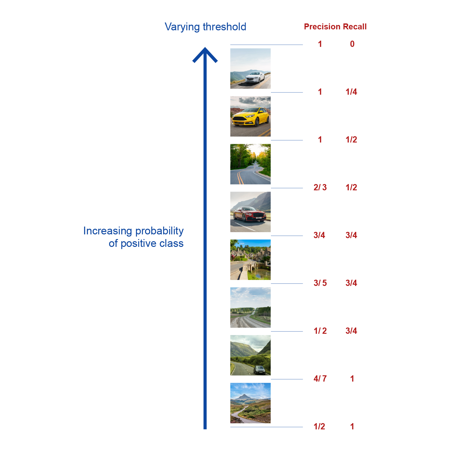
Figure 2. Precision and recall for varying probability threshold.
A stack of 8 images, some of which depict a car. The images are ordered by the probability of being a car, as output by a classifier. The 9 distinct precision and recall values obtained by setting increasing threshold values from 0 to 1 are shown alongside the stack.
The corresponding PR curve looks like this:

Figure 3. Precision-recall curve corresponding to the varying threshold values tabulated in Figure 2.
A graph with precision values plotted on the y-axis corresponding to the recall values on the x-axis. This is the precision-recall curve.
It is often convenient to summarise the value of precision and recall as a single value. The F-score is the harmonic mean of precision and recall, given by:
The reason for using the harmonic mean instead of the arithmetic mean is to penalise situations where either the precision or recall are low. This can be seen from the following visualisation of F-scores for all combinations of precision and recall values.

Precision and recall in multiclass classification
Precision and recall are also used as a performance measure with respect to individual classes in multi-class classification. In the three class example at the start, we can compute recall and precision values for the truck class just as we did for the positive class in binary classification:
These statistics are particularly useful when we have an unbalanced dataset, with very different numbers of examples in each class. Consider for example the following confusion matrix:
| Predicted class | ||||
|---|---|---|---|---|
| Car | Bicycle | Truck | ||
| Actual class | Car | 1000 | 5 | 5 |
| Bicycle | 10 | 0 | 0 | |
| Truck | 10 | 0 | 0 | |
In this case there are many more cars than trucks and bicycles. The classifier makes the wrong prediction for every truck and bicycle, yet the accuracy is high:
In this case, the accuracy is misleading. Fortunately the recall for the truck and bicycle classes show that the performance on these two classes is poor.
A good way to summarise the performance with unbalanced datasets is to take the mean of the recall values for each class. This is known as the balanced accuracy.
For the example above, the balanced accuracy is given by:
This is very different from the accuracy value and a more representative measure of performance in this case.
When there is an equal number of examples in each class, the balanced accuracy is identical to the accuracy.